Adding a Background field to Langmuir Turbulence example

[ammtD]

Hello,

I am trying to set the Langmuir Turbulence simulation in a background velocity and stratification.

The ultimate goal is to implement an idealized U(z) and B(z). However, taking small steps to get this to work, I start with adding the line

``Ufield(x,y,z,t) = 0.2*z

and

model = NonhydrostaticModel(architecture = CPU(),  advection = WENO5(),   timestepper = :RungeKutta3,
                   grid = grid,   background_fields = (u=Ufield,),    tracers = (:b,),     buoyancy = BuoyancyTracer(),
              coriolis = coriolis,    closure = AnisotropicMinimumDissipation(),  stokes_drift = UniformStokesDrift(∂z_uˢ=dus_dz),
    boundary_conditions = (u=u_bcs, b=b_bcs), )

For the rest no changes are made w.r.t. the example.

The first model step takes a lot of time to execute, and afterwards it directly crashes, because of the occurrence of NaNs in t and u fields.

@ Oceananigans.Simulations C:\Users\Owner\.julia\packages\Oceananigans\W8B0n\src\Simulations\run.jl:179
┌ Info: i: 0010, t: 8.250 minutes, Δt: NaN years, umax = (NaN, NaN, NaN) ms⁻¹, wall time: 4.892 minutes
└ @ Main In[1]:93
 Info: i: 0020, t: NaN years, Δt: NaN years, umax = (NaN, NaN, NaN) ms⁻¹, wall time: 4.915 minutes
└ @ Main In[1]:93

Any thoughts? I can add the script I am using, if that's helpful?
I suspect that there may be a mismatch between this background field, and initialization of the resolved fields and/or boundary conditions?

Thanks in advance!

[glwagner]

Hi @ammtD ! Can you share your whole script? We need that in order to figure out what this issue might be, and also to run the script ourselves to debug the problem.

I'm going to convert this issue to a discussion!

[glwagner]

I think the probable reason for NaN is because the time-step is too long.

I can't know for sure without seeing the grid, but assuming you are using the same grid from the Oceananigans, example, then with U(x, y, z, t) = 0.2 * z, the current at the bottom of the domain is 0.2 * 64 = 12.8 m/s -- quite fast. So with 4m grid spacing (which is used in the example, but you may have changed it) a time-step with CFL=1 would be around Δt = 4 / 12.8 = 0.31 seconds.

I stripped down the example to produce this:

using Oceananigans
using Oceananigans.Units: minute, minutes, hours
using Oceananigans.BuoyancyModels: g_Earth
using GLMakie

grid = RectilinearGrid(size=(32, 32, 32), extent=(128, 128, 64))
coriolis = FPlane(f=1e-4) # s⁻¹

amplitude  = 0.8 # m
wavelength = 60 # m
wavenumber = 2π / wavelength # m⁻¹
frequency  = sqrt(g_Earth * wavenumber) # s⁻¹

const vertical_scale = wavelength / 4π
const Uˢ = amplitude^2 * wavenumber * frequency # m s⁻¹

uˢ(z) = Uˢ * exp(z / vertical_scale)
@inline ∂z_uˢ(z, t) = 1 / vertical_scale * Uˢ * exp(z / vertical_scale)

Qᵘ = -3.72e-5 # m² s⁻², surface kinematic momentum flux
Qᵇ = 2.307e-9 # m³ s⁻², surface buoyancy flux
N² = 1.936e-5 # s⁻², initial and bottom buoyancy gradient

u_boundary_conditions = FieldBoundaryConditions(top = FluxBoundaryCondition(Qᵘ))
b_boundary_conditions = FieldBoundaryConditions(top = FluxBoundaryCondition(Qᵇ),
                                                bottom = GradientBoundaryCondition(N²))

@inline U(x, y, z, t) = 0.2 * z

model = NonhydrostaticModel(; grid, coriolis,
                            advection = WENO5(),
                            timestepper = :RungeKutta3,
                            tracers = :b,
                            buoyancy = BuoyancyTracer(),
                            closure = AnisotropicMinimumDissipation(),
                            stokes_drift = UniformStokesDrift(; ∂z_uˢ),
                            background_fields = (; u = U),
                            boundary_conditions = (u=u_boundary_conditions, b=b_boundary_conditions))


Ξ(z) = randn() * exp(z / 4)
initial_mixed_layer_depth = 33 # m
stratification(z) = z < - initial_mixed_layer_depth ? N² * z : N² * (-initial_mixed_layer_depth)
bᵢ(x, y, z) = stratification(z) + 1e-1 * Ξ(z) * N² * model.grid.Lz

u★ = sqrt(abs(Qᵘ))
wᵢ(x, y, z) = u★ * 1e-1 * Ξ(z)
set!(model, u=wᵢ, w=wᵢ, b=bᵢ)

simulation = Simulation(model, Δt=0.1, stop_iteration=1000)

wizard = TimeStepWizard(cfl=1.0, max_change=1.1, max_Δt=0.3)
simulation.callbacks[:wizard] = Callback(wizard, IterationInterval(10))

print_progress(sim) = @info string("Iter: ", iteration(sim), ", time: ", prettytime(sim),
                                   ", max|w|: ", maximum(abs, sim.model.velocities.w))
simulation.callbacks[:progress] = Callback(print_progress, IterationInterval(10))

simulation.output_writers[:fields] =
    JLD2OutputWriter(model, merge(model.velocities, model.tracers),
                     schedule = IterationInterval(100),
                     prefix = "langmuir_turbulence",
                     force = true)

run!(simulation)

filepath = "langmuir_turbulence.jld2"
w_ts = FieldTimeSeries(filepath, "w")
Nt = length(w_ts.times)

fig = Figure()
ax = Axis(fig[1, 1])
slider = Slider(fig[2, 1], range=1:Nt, startvalue=1)
n = slider.value

wn = @lift interior(w_ts[$n], :, 1, :)
heatmap!(ax, wn)

record(fig, "langmuir_turbulence.mp4", 1:Nt, framerate=24) do nn
    n[] = nn
end

which runs with an initial time-step of Δt = 0.1. I've also set max_Δt = 0.3 in the TimeStepWizard (since it doesn't use background fields in its CFL calculation at the moment). Note that this mixes much faster than the example... check it out:

langmuir_turbulence.mp4

[ammtD]

Hi Greg.
Yes, I was using the same setup as you just used there. Thanks for trying this out.
And sorry....I guess this was the obvious problem; I am new to modelling and had not been mindful of changing the cfl and timestepper.
After a discussion with my mentors we came to the same conclusion; Our idealized current with max(abs(u))=1.5 m/s ( set as initial condition for now, I'll try the background-field setup later today) requires a small reduction of the CFL, and a timestep of ~ 1s.

[ammtD]

Ok, so rather than

B(x, y, z, t, p) = - p.α * p.f * y + p.N^2 * z
B_field = BackgroundField(B, parameters=basic_state_parameters)

as is done in the Eady Turbulence example, you'd use @inline B(x, y, z, t, p) ?
And leave the B_field definition as is ?

[glwagner]

Yes, @inline only affects function definitions.

Might be good to add @inline to the example! Feel free to PR!

[ammtD]

I'd be interested to see the differences between using BackgroundField and not!

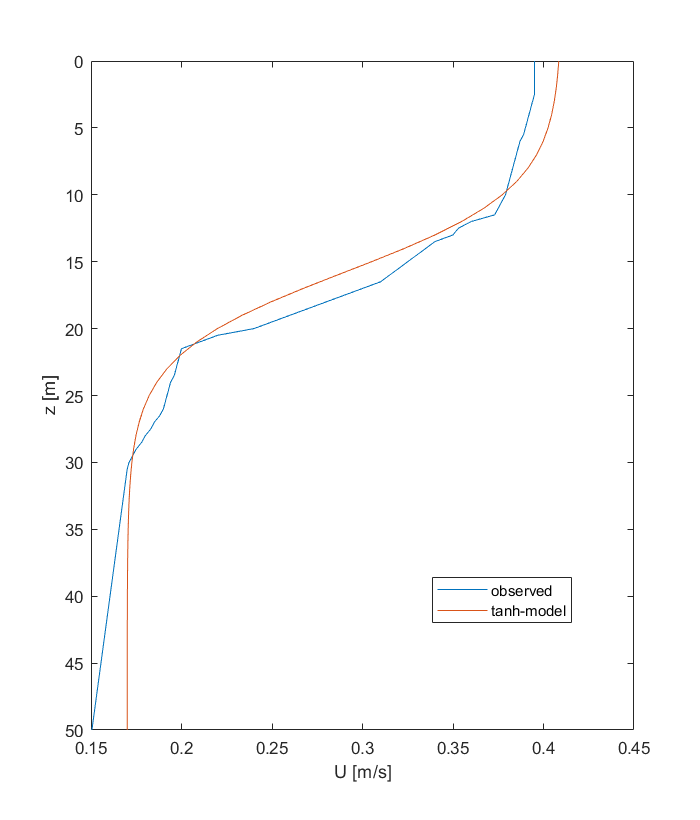
So, I am back at this, after having updated to the most recent version of Oceananigans.jl.

Following on our communication on Slack, I was trying to set an array as a background field.

Ubg_array=repeat(reshape(Uj,1,1,Nz), Nx , Ny, 1);
Ubg= XFaceField(grid)    # CenterField(grid)
set!(Ubg, Ubg_array); 

model = NonhydrostaticModel(; grid, ....., background_fields = (; u = Ubg))

But I found this doesn't go well.... the model ran but quickly simulated velocities to be on the order of 20 m/s....(background velocity is only 0.15 - 0.5 m/s.

I fear that the attempted 'velocity-profile' Uj used in Ubg_array , is not smooth enough.... some differential may screw up the simulation therefore. Would you agree (see image)?

I am running the model again now using an approximation of Uj (a tanh-function), which seems to solve the issue.

[glwagner]

That's interesting. Seems like a plausible hypothesis, but I'm not sure. Did you test whether the results depended on time step?

[ammtD]

The code runs with Δt=2.0, max_ Δt=5.0seconds for either case, increasing max_Δt by much makes either crash. But I haven't extensively tested the limits (and whether they depend on how I define the bg-field) .