1. Typify model into PA or PAD based on the purpose and in-hand data

[hyunjimoon]

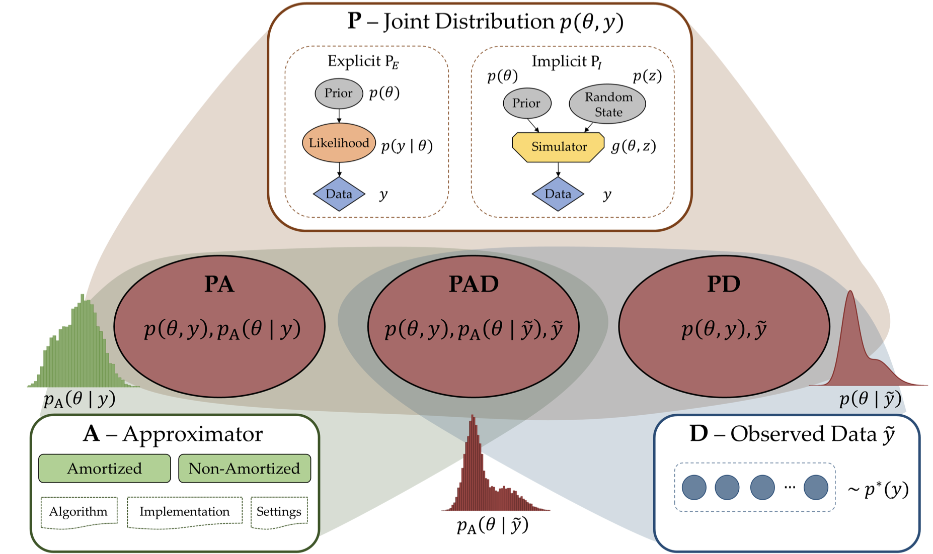
Considering expanding model workflow would always bump into the boundary of deterministic parameter, classifying deterministic and stochastic model would have little value. On the other hand, empirical vs theoretical i.e. using observed data or not matters which can be uniformly expressed with PA and PAD modeling in this paper. [1] As ode integrator is embedded for ode modeling, I assumed PD which doesn't involve approximator cannot exist from the figure below.

Below are the list of each model's character from @tomfid's SIG talk "Data and Uncertainty in System Dynamics" and @hazhirr's class on Brining data into Dynamic model.

PA modeling

• If model structure is to follow real-world structures underlying the problem, qualitative data is needed for building it
• Insights can be generated before starting to use numerical data
• Save lots of time on collection, preprocessing and calibration
• Potentially reallocate to client interaction, robustness testing and scenario experimentation
• Less cognitive load for participants

PAD modeling

• Uncertainties in parameter values can only be settled with empirical data
• Many theoretical and practical implications depend on these parameters, e.g. any cost-benefit requires reliable estimates of both costs and benefits, and estimates of uncertainty around both
• No learning about the data, or from the data directly
• No contribution to model quality from tests against data
• Hard to verify that asserted reference modes or decision structures match reality
• Less face validity of historical runs
• Difficulty understanding the gaps between a priori parameter values and most plausible values, given the model
• No objective basis for parameter values or confidence bounds
• Hard to understand the joint uncertainty of a parameter set

Decision-based Bayesian Workflow

Building on the above, I drafted a three step model-building scenario. Data is arrays of vectors of observed, Draws is arrays of vectors of sampled unobserved, Demand is a functional form of policy. All of them can be dynamic i.e. function of time, but we restrict Demand to time-heterogenous. This is based on Yaman's explanation, "A policy is expressed in general by a policy equation, not by a single parameter. Policy equations naturally have policy parameters. Can policy analysis be carried out by simply changing values of policy parameters? The answer is: not always, but to a great extent. In more advanced policy analysis, we need to change the forms of the policy equations, not just parameter values. But I now strongly suggest that you ignore this at this point and focus on parameters values of fixed policy equations.

1. Verify Draws-Demand

We start from PA modeling. Given P (joint distribution of observed and unobserved) generated either explicitly (e.g. Bayesian learning) or implicitly (e.g. deep learning), we experiment within the following:

• data: synthetic
• data2draws: assuming asymptotic, unbiased, estimation methods e.g. HMC, filtering methods
• demand: stiff binary

2. Validate Data - [Draws - Demand] with testing-framed demand

Then we proceed to PAD modeling by adding D i.e. observed, real-world data. Given D, we experiment within the following:

• demand: flexible binary (more-than-two allowed by re-formulating into binary trees)
• data2demand: Bayes factor simulation-based calibration and indirect inference
• draws: possibly biased approximators e.g. simulation-based inference, BayesFlow.

We reverse engineer the first iteration by asking, "to make our demand noise-resilient, what form should our demand be, what data is needed, and what estimation method can do this most efficiently"? This order is common in Bayesian inference where we first build the generator then do the inference conditional on the data. Working in both directions is the benefit of generative model (e.g. Bayesian) which operates on joint space of observed and unobserved. Using this benefit, we argue the best practice of model building is to first make the rough mockup from data to demand then building up from the demand's end. For instance, the effect of new data on demand can be forwardly-simulated, then compared to inform us the best data. This spirit is similar to Bayesian optimization. However, unlike their description of "taking human out of the loop", we aim to design human-machine interface. In practice, human's form of demand, or activation function in Bayesian optimization, becomes clearer during the model building iteration.

Parsimoniously constructed graphs with appropriate level of parameter uncertainty (i.e. identifiable structure with tight prior distribution) will facilitate the inverse procedure by preventing degeneracy in posterior space.

On top of the above listed value of PAD modeling, Jeroen and I identified two additional benefits related to tipping points:

• prevent fixed value of parameters cross the tipping boundaries
• remove unrealistic attractor

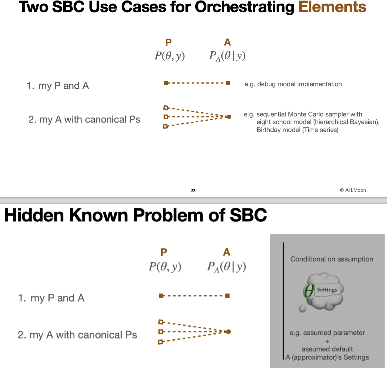
Jeroen's poster in ISDC 2022, Sustainable consumption transformations: Should we mobilize the young generation? below illustrates the two. Refer to Struben22_SustainTrans.pdf inref folder (requested to Jeroen to share reference link (and with generosity his codes).

First, the model qualification test outcome (pass/fail) depends on the value assumed parameter is conditioned upon. Like a water's boiling point (100 degree at 1 atm), tipping points boundary is unavoidable. The least we can do is to move our demand (mostly binary, at most finite) away from these sensitive borders. The easiest remedy is to adjust the fixed value of assumed parameter as this sometimes is modeler's rough assumption. However, changing estimated parameter's prior distribution or prior parameter can be another remedy, followed by changing model parameterization or components. Even collecting more data are possible and recommended if this can make our demand more resilient.

Jeroen's poster on aging model illustrates two attractors in the phase space; however, this analysis is based on the fixed value of assumed parameter (noted as green in his poster, e.g. active life duration). Fixing can be problematic in two ways: first in calibration then in analysis. Regarding calibration, the model that passed quality test when conditioned on at 20 can fail the test at = 30. In other words, the same model qualified in 1900s (or at the time when active life duration was 20 years) becomes outdated as society evolved to the era of longer active life duration. Considering both real data and parameter for calibration is well discussed in the upcoming paper on simulation-based calibration. Second, even if the model passed the quality test, under different conditioning, the analysis (two attractors in phase space) may completely change. There may be one or three attractors for instance, affecting the downstream policy proposal.

Assumed-value of nuisance parameter affecting the test result is problematic but unavoidable as we can't afford full-Bayesian model where uncertainty is imbued to every parameter. Like a Pirate Roulette game, we should pray each time that our slice of fixed parameter hyperplane does not cross the tipping points. Inference helps us in this respect as we can alternately focus on different parameters by switching back and forth between estimated parameter and assumed parameter. This zig-zag learning like that of Gibbs sampling is suboptimal but can help keep modelers away from borders by providing a more global view of the decision geometry.

Second, is to argue the state value of a particular attractor is not realistic. Globally it may be the bimodal but if the scale of state for the second mode is out of bounds we may as well consider it unimodal. This allows us to save considerable amount of further analysis (Analysis of tipping behavior from the poster) by precluding certain scenarios. However, both known and unknown bias should be acknowledged as data in hand may not be the just representation of population.

• Alluded above in the second benefit of removing multi-modality, mapping boundary of tipping point in state space with that of multimodality in parameter space is my main research interest and I have listed here with four examples collected from @tomfid and @hazhirr's writing.

• For "Testing-framed demand" refer to "Testing-framed decisions" in 2. Typify parameters in syntax-semantic with colors, units, bounds #7.

3. Prescribe policy parameter with [Data - [Draws - Demand]]

For the final iteration, we invite policy and behavior on top of PAD calibration flow we constructed in 1 and 2. Given function of Demand and observed data D, we experiment within the following (discussion needed):

• demand: potentially non-discrete
• data to demand: Bayes factor simulation-based calibration and indirect inference
• draws: posterior approximators from simulation-based inference e.g. BayesFlow
  The last two is equivalent to above 2, the only difference being 2 is on physical parameter of our existing system (e.g. disease and community parameters) whereas 3 is what imaginary parameter (or at least implementation in process) for management (e.g. policy levers). Example of this parameter classification can is detailed in Colored diagrams section of 2. Typify parameters in syntax-semantic with colors, units, bounds #7.

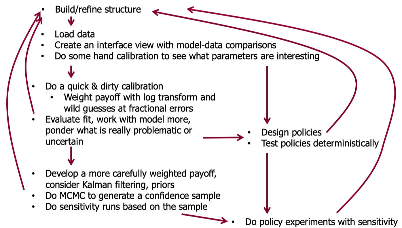
@tomfid's suggested parallel workflow of calibration and decision in the diagram below, which I view as coflow of 2 and 3.

Both parameteric and nonparameteric approach exist to address these non-binary and sometimes continuous objects. We visit seminal works by John, Tom, Rogelio, Andrew, Yaman, Erling and seek ways to connect their softwares for the automated Bayesian workflow. For detail, refer to Supply of SilkRoad project.

Specific topics are to be decided but the following are relevant:

• Indirect structure testing: Extreme condition hypothesis testing
• Sensitivity analysis (by behavior pattern space): Behavior pattern sensitivity with respect to parameter changes
• Model calibration: Automated parameter calibration based on input (real) behavior patterns
• Policy analysis and design: Policy parameter(s) specification based on desired behavior patterns
• Discuss similarity and difference in discriminate, cluster, classify, outlier-removal from optimization's three steps viewpoint (recognize, evaluate, optimize)

[hyunjimoon]

Using data, transformed data, generated quantities block well, we can control different moving parts of optimization, designing P and A for instance. The chart below from Moon20_LetsSBC_GelmanIntern compares the difference. Two use cases of SBC builds on this result which is shown in p.33 of [actionable workflow] (https://github.com/Data4DM/BayesSD/blob/master/DailyDigest/Moon22_ActionableWorkflow.pdf) talk slide. It walks you through PAD with examples, two usecases, and hidden known problems.