Process Graph Building
As with the change of the openeo versions from 0.3.x to 0.4.x the process graph structure was completely overhauled. This mainly due to the fact that those graphs and much redundancy and it was not really possible to reuse intermediate results in different processes other than recalculating everything again. Also the change of the intentional data structure of multi-dimensional data cubes and the associated focus on reducing and aggregating of dimensions by using functions (callbacks) to control the reduction behavior pushed into this new leaner representation of process graphs introduced by the 0.4.x openeo API.
The R client supports this new process graph handling with versions >= 0.4.1 and the graph creation is only handled by the process graph builder which was introduced with version 0.2.1. The old functions process and collection are no longer available - collection was mainly removed since the openeo processes offer a load_collection function which would then be a process.
During the development it became clear that we need an object-oriented programming style to realize the new process graph. The main reasons are that
- we have quite a lot of typed objects as argument values which relates to inheritance
- we do not want to lose overview (have private and public functions for objects)
- we want objects to behave similar, but in some cases differently (type checking, validation, serialization, etc.)
Those are some of the reasons why we modelled the process graph handling as R6 classes.
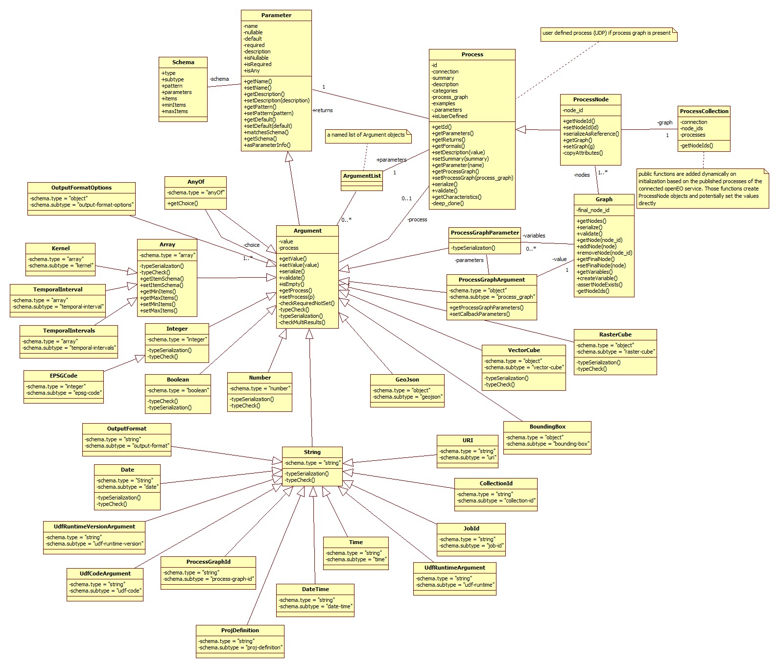
0.4.x process graph model
The main take home message here is that a graph consists of process nodes which are derived from processes and extended with a node id and a special serialization. Parameters keep the information about the parameter of a process and the derived argument object keeps additionally the value which will be set by the user.
The process graph builder is created by querying the back-end for all available collections and processes. The information is received as JSON objects. From the collection response the collection ids are extracted and stored in a named list at graph$data. The lists names and the values are the same - the collection id. The processes response is parsed and translated into Process objects with Argument objects instead of Parameter objects. Those Process objects are registrated within functions on the Graph object (the function process_graph_builder() returns a Graph object). The parameter names of this process creator functions are the same as those specified by the back-end and if the values are set, then they are also set in the corresponding Argument object of the Process.
con = connect(host = "http://demo.openeo.org", version="0.4.2",user = "some_user",password = "some_pwd",login_type = "basic")
graph = con %>% process_graph_builder()

class(graph)
## [1] "Graph" "R6"
head(graph$data,5)## $`AAFC/ACI`
## [1] "AAFC/ACI"
##
## $`ASTER/AST_L1T_003`
## [1] "ASTER/AST_L1T_003"
##
## $`AU/GA/AUSTRALIA_5M_DEM`
## [1] "AU/GA/AUSTRALIA_5M_DEM"
##
## $`CAS/IGSNRR/PML/V2`
## [1] "CAS/IGSNRR/PML/V2"
##
## $`CIESIN/GPWv4/population-count`
## [1] "CIESIN/GPWv4/population-count"
graph$getNodes()## list()
graph$reduce()## <ProcessNode>
## Inherits from: <Process>
## Public:
## clone: function (deep = FALSE)
## getCharacteristics: function ()
## getFormals: function ()
## getId: function ()
## getNodeId: function ()
## getParameter: function (name)
## getParameters: function ()
## getReturns: function ()
## initialize: function (node_id = character(), process)
## parameters: active binding
## serialize: function ()
## serializeAsReference: function ()
## setDescription: function (value)
## setNodeId: function (id)
## setParameter: function (name, value)
## validate: function (node_id = NULL)
## Private:
## .parameters: list
## categories:
## copyAttributes: function (process)
## deep_clone: function (name, value)
## description:
## examples: list
## id: reduce
## node_id: reduce_GEXRB8006P
## parameter_order: list
## returns: list
## summary: Reduce dimensions
In this example we are going to calculate the minimum NDVI and apply a linear stretch into the byte value domain to store and view the results as PNG. The file format PNG works only with bytes - otherwise the image would be pitch black (NDVI value range is between -1 and 1).
First, we prepare a graph with the process graph builder and then we define the data we want to load. In this case the load_collection function already offers parameter to subset the collection. If this back-end would not offer this, we would have to chain the individual functions afterwards - like filter_bbox, filter_time, etc.
graph = con %>% process_graph_builder()
data1 = graph$load_collection(id = graph$data$`COPERNICUS/S2`,
                              spatial_extent = list(west=-2.7634,south=43.0408,east=-1.121,north=43.8385),
                              temporal_extent = c("2018-04-30","2018-06-26"),bands = c("B4","B8"))
Up next, extract the bands that are referenced with the band names that are used in band dimension of the data cube and pass those to the normalized_difference process.
b4 = graph$filter_bands(data = data1,bands = "B4")
b8 = graph$filter_bands(data=data1,bands = "B8")

ndvi = graph$normalized_difference(band1 = b4,band2 = b8)
The next part will be a bit trickier. In order to find the minimum value over time, we have to reduce the time dimension. This means we more or less get rid of the time dimension by applying a callback containing only a minimum function. It will work the way that the callback function is applied on every cell with the data of its temporal dimension aggregate. Now, in the client we will create a callback based on the parent process (the process providing data for the callback) and the particular parameter name, but first we can find out which parameter has to receive the callback by omitting the parameter parameter. Since the callback is also a graph it can be similarly build up as we did before. But the data injection works different in this case. The callback graph is already configured that the callback parameters are already available under cb_graph$data. When the process graph is finished we need to set the result node - the node that will return the result for the potential next process.
con %>% callback(graph$reduce())## Parameter that expect a callback: reducer
reducer = graph$reduce(data = ndvi,dimension = "temporal")

cb_graph = con %>% callback(reducer,parameter = "reducer")

cb_graph$min(data = cb_graph$data$data) %>% cb_graph$setFinalNode()
## [1] TRUE
To apply the linear stretch we will litterally apply the function to each cell. This translates into modifying single values. Therefore we are going to create another callback.
apply_linear_transform = con %>% graph$apply(data = reducer)

cb2_graph = con %>% callback(apply_linear_transform, "process")

cb2_graph$linear_scale_range(x = cb2_graph$data$x, inputMin = -1, inputMax = 1,outputMin = 0,outputMax = 255) %>%
  cb2_graph$setFinalNode()
## [1] TRUE
At the end we save the result as PNG file and also mark the result node of the graph.
graph$save_result(data = apply_linear_transform,format = "png") %>% graph$setFinalNode()## [1] TRUE
graph## {
## "load_collection_QPJZO9671T": {
## "process_id": "load_collection",
## "arguments": {
## "id": "COPERNICUS/S2",
## "spatial_extent": {
## "west": -2.7634,
## "south": 43.0408,
## "east": -1.121,
## "north": 43.8385
## },
## "temporal_extent": [
## "2018-04-30",
## "2018-06-26"
## ],
## "bands": [
## "B4",
## "B8"
## ]
## }
## },
## "filter_bands_EGSJI4233I": {
## "process_id": "filter_bands",
## "arguments": {
## "data": {
## "from_node": "load_collection_QPJZO9671T"
## },
## "bands": [
## "B4"
## ]
## }
## },
## "filter_bands_BQJPX9753H": {
## "process_id": "filter_bands",
## "arguments": {
## "data": {
## "from_node": "load_collection_QPJZO9671T"
## },
## "bands": [
## "B8"
## ]
## }
## },
## "normalized_difference_XWWKP1447Z": {
## "process_id": "normalized_difference",
## "arguments": {
## "band1": {
## "from_node": "filter_bands_EGSJI4233I"
## },
## "band2": {
## "from_node": "filter_bands_BQJPX9753H"
## }
## }
## },
## "reduce_LANDI3801V": {
## "process_id": "reduce",
## "arguments": {
## "data": {
## "from_node": "normalized_difference_XWWKP1447Z"
## },
## "reducer": {
## "callback": {
## "min_GZVHW5850J": {
## "process_id": "min",
## "arguments": {
## "data": {
## "from_argument": "data"
## }
## },
## "result": true
## }
## }
## },
## "dimension": "temporal"
## }
## },
## "apply_FQWGW3646X": {
## "process_id": "apply",
## "arguments": {
## "data": {
## "from_node": "reduce_LANDI3801V"
## },
## "process": {
## "callback": {
## "linear_scale_range_QLIOM3833L": {
## "process_id": "linear_scale_range",
## "arguments": {
## "x": {
## "from_argument": "x"
## },
## "inputMin": -1,
## "inputMax": 1,
## "outputMin": 0,
## "outputMax": 255
## },
## "result": true
## }
## }
## }
## }
## },
## "save_result_DQPBZ6428V": {
## "process_id": "save_result",
## "arguments": {
## "data": {
## "from_node": "apply_FQWGW3646X"
## },
## "format": "png"
## },
## "result": true
## }
## }
Strictly speaking callbacks are nothing else than sub process graphs. However, callbacks differ in terms of data injection. On the back-end data is pushed into the corresponding entry process that claims to receive a callback parameter (or in the R client terminology a callback value), whereas the usualprocess graph loads loads the data via an dedicated process like load_collection and the process results are passed on. Those callback parameter are usually vectors or two single values.
The following code snippet shows data injected to the main process graph, e.g. loading a data collection.
load_collection = graph$load_collection(id = graph$data$`COPERNICUS/S2`,
                              spatial_extent = list(west=-2.7634,south=43.0408,east=-1.121,north=43.8385),
                              temporal_extent = c("2018-04-30","2018-06-26"),bands = c("B4","B8"))
jsonlite::toJSON(load_collection$serialize(),auto_unbox = TRUE,pretty=TRUE)
## {
## "process_id": "load_collection",
## "arguments": {
## "id": "COPERNICUS/S2",
## "spatial_extent": {
## "west": -2.7634,
## "south": 43.0408,
## "east": -1.121,
## "north": 43.8385
## },
## "temporal_extent": [
## "2018-04-30",
## "2018-06-26"
## ],
## "bands": [
## "B4",
## "B8"
## ]
## }
## }
The next two snippets show the two types of callback parameter - first the array input, second two values as input.
cb_graph$data## $data
## {
## "from_argument": "data"
## }
cb2_graph$data## $x
## {
## "from_argument": "x"
## }
## $y
## {
## "from_argument": "y"
## }
The callback parameter can be thought of the signature of the callback function - meaning if we have a single data object as callback parameter we can assume in almost all cases that the data type is an array / vector.
The callback handling definition is under development right now (> v0.5). So in the future the callback creation becomes as easy as defining a function in R. The openeo package will do the transformation into a valid process graph internally.
The graph$data field contains the data available to a graph. In the case where the graph is build regularly with the process_graph_builder() the data corresponds with the available collections on the back-end. In callback graphs data will be filled by the arguments callback parameter.
Processes are received from the back-end in a particular format. It contains general information about the process, but more important information about its parameter, e.g. name, order and type/format.
toJSON(con %>% describe_process("filter_bands"),force=TRUE,auto_unbox = TRUE,pretty = TRUE)## {
## "id": "filter_bands",
## "summary": "Filter the bands by name",
## "description": "Filters the bands in the data cube so that bands that don't match any of the criteria are dropped from the data cube. The data cube is expected to have only one dimension of type `bands`. Fails with a `DimensionMissing` error if no such dimension exists.\n\nThe following criteria can be used to select bands:\n\n* `bands`: band name (e.g. `B01` or `B8A`)\n\n**Important:** The order of the specified array defines the order of the bands in the data cube, which can be important for subsequent processes. If multiple bands are matched by a single criterion (e.g. a range of wavelengths), they are ordered alphabetically by band names. Bands without names have an arbitrary order.",
## "categories": [
## "filter"
## ],
## "gee:custom": true,
## "parameter_order": [
## "data",
## "bands"
## ],
## "parameters": {
## "data": {
## "description": "A data cube with bands.",
## "schema": {
## "type": "object",
## "format": "raster-cube"
## },
## "required": true
## },
## "bands": {
## "description": "A list of band names.\n\nThe order of the specified array defines the order of the bands in the data cube.",
## "schema": {
## "type": "array",
## "items": {
## "type": "string",
## "format": "band-name"
## }
## },
## "required": true
## }
## },
## "returns": {
## "description": "A data cube limited to a subset of its original bands. Therefore, the cardinality is potentially lower, but the resolution and the number of dimensions are the same as for the original data cube.",
## "schema": {
## "type": "object",
## "format": "raster-cube"
## }
## },
## "exceptions": {
## "DimensionMissing": {
## "message": "A band dimension is missing."
## }
## },
## "links": [
## {
## "rel": "about",
## "href": "https://github.com/radiantearth/stac-spec/tree/master/extensions/eo#common-band-names",
## "title": "List of common band names as specified by the STAC specification"
## }
## ]
## }
All those information are parsed and interpreted in order to create a suitable process representation in R. Those processes will be registered as constructor functions on the graph. This means by calling the function a parsed process will be copied, turned into a process node and added to the process graph.
graph$filter_bands## function (data = NA, bands = NA)
## {
## process = processes[[13]]$clone(deep = TRUE)
## node_id = .randomNodeId(process$getId(), sep = "_")
## while (node_id %in% private$getNodeIds()) {
## node_id = .randomNodeId(process$getId(), sep = "_")
## }
## arguments = process$parameters
## this_param_names = names(formals())
## this_arguments = lapply(this_param_names, function(param) get(param))
## names(this_arguments) = this_param_names
## lapply(names(this_arguments), function(param_name, arguments) {
## call_arg = this_arguments[[param_name]]
## arguments[[param_name]]$setValue(call_arg)
## }, arguments = arguments)
## node = ProcessNode$new(node_id = node_id, process = process)
## private$nodes = append(private$nodes, node)
## return(node)
## }
## <bytecode: 0x000000001c8b5a50>
## <environment: 0x0000000012c91580>
Now if we want to apply the graph easier to different data sets, we can introduce variables and store this parametrized graph to the back-end. If the back-end offers the process to load process graphs we then can execute the parametrized graph by filling in the variables. If we don't fill in the variable values, the default value is assumed and if the default is not set and the graph shall be executed on the back-end it will result in an error at the back-end.
We can either use the variables directly during the graph creation as argument values or we can replace some of the values afterwards. Since the first part is quite obvious to do, we will give an example where we create three variables for the collections and the two bands and replace them at the afore created process graph of the Example section.
collection_id = graph$createVariable(id = "collection",description = "The collection id of a cube containing at least a red and a near infrared band",type = "string",default = "COPERNICUS/S2")

red_band = graph$createVariable(id = "red_band",description="The band name of the red band",type="string",default="B4")

nir_band = graph$createVariable(id = "nir_band",description="The band name of the NIR band",type="string",default="B8")

names(variables(graph))
## [1] "collection" "red_band" "nir_band"
You can fetch the variables also at a later stage, by using variables on the graph object. The variables here are defined in this context and may or may not have been used in the graph.
graph$setArgumentValue(node_id = data1$getNodeId(), parameter = "id", value = collection_id)
graph$setArgumentValue(node_id = data1$getNodeId(), parameter = "bands", value = NULL)


graph$setArgumentValue(node_id = b4$getNodeId(), parameter="bands", value=red_band)
graph$setArgumentValue(node_id = b8$getNodeId(), parameter="bands", value=nir_band)

graph
## {
## "load_collection_QPJZO9671T": {
## "process_id": "load_collection",
## "arguments": {
## "id": {
## "variable_id": "collection",
## "description": "The collection id of a cube containing at least a red and a near infrared band",
## "type": "string",
## "default": "COPERNICUS/S2"
## },
## "spatial_extent": {
## "west": -2.7634,
## "south": 43.0408,
## "east": -1.121,
## "north": 43.8385
## },
## "temporal_extent": [
## "2018-04-30",
## "2018-06-26"
## ]
## }
## },
## "filter_bands_EGSJI4233I": {
## "process_id": "filter_bands",
## "arguments": {
## "data": {
## "from_node": "load_collection_QPJZO9671T"
## },
## "bands": {
## "variable_id": "red_band",
## "description": "The band name of the red band",
## "type": "string",
## "default": "B4"
## }
## }
## },
## "filter_bands_BQJPX9753H": {
## "process_id": "filter_bands",
## "arguments": {
## "data": {
## "from_node": "load_collection_QPJZO9671T"
## },
## "bands": {
## "variable_id": "nir_band",
## "description": "The band name of the NIR band",
## "type": "string",
## "default": "B8"
## }
## }
## },
## "normalized_difference_XWWKP1447Z": {
## "process_id": "normalized_difference",
## "arguments": {
## "band1": {
## "from_node": "filter_bands_EGSJI4233I"
## },
## "band2": {
## "from_node": "filter_bands_BQJPX9753H"
## }
## }
## },
## "reduce_LANDI3801V": {
## "process_id": "reduce",
## "arguments": {
## "data": {
## "from_node": "normalized_difference_XWWKP1447Z"
## },
## "reducer": {
## "callback": {
## "min_GZVHW5850J": {
## "process_id": "min",
## "arguments": {
## "data": {
## "from_argument": "data"
## }
## },
## "result": true
## }
## }
## },
## "dimension": "temporal"
## }
## },
## "apply_FQWGW3646X": {
## "process_id": "apply",
## "arguments": {
## "data": {
## "from_node": "reduce_LANDI3801V"
## },
## "process": {
## "callback": {
## "linear_scale_range_QLIOM3833L": {
## "process_id": "linear_scale_range",
## "arguments": {
## "x": {
## "from_argument": "x"
## },
## "inputMin": -1,
## "inputMax": 1,
## "outputMin": 0,
## "outputMax": 255
## },
## "result": true
## }
## }
## }
## }
## },
## "save_result_DQPBZ6428V": {
## "process_id": "save_result",
## "arguments": {
## "data": {
## "from_node": "apply_FQWGW3646X"
## },
## "format": "png"
## },
## "result": true
## }
## }