Wouter van Atteveldt & Kasper Welbers 2022-01
- Introduction
- Obtaining and exploring data
- Training and test data
- A naive Bayes model
- SVM: Tuning models, recipes, and workflows
- Parameter tuning
- What’s next?
In this tutorial, we use the following packages: (note that there is no need to install packages again if you previously installed them)
install.packages("tidyverse")
install.packages("tidymodels")
install.packages("naivebayes")
install.packages("kernlab")
install.packages("skimr")
install.packages("corrplot")
The main library we use is tidymodels, which (like tidyverse) is a
‘meta-package’ that includes various packages to do machine learning.
This tutorial will take you through the most important, including:
- rsample to split data into train/test sets
- parsnip to do the actual machine learning
- recipes to create preprocessing / feature encoding ‘recipes’
- workflows ` to encode the whole workflow of training and testing models
- tune to do hyperparameter tuning
This might sound daunting, but there is method to the madness. This image (from the free online book (Tidyverse Skills for Data Science)[https://jhudatascience.org/tidyversecourse/]) gives a nice overview:
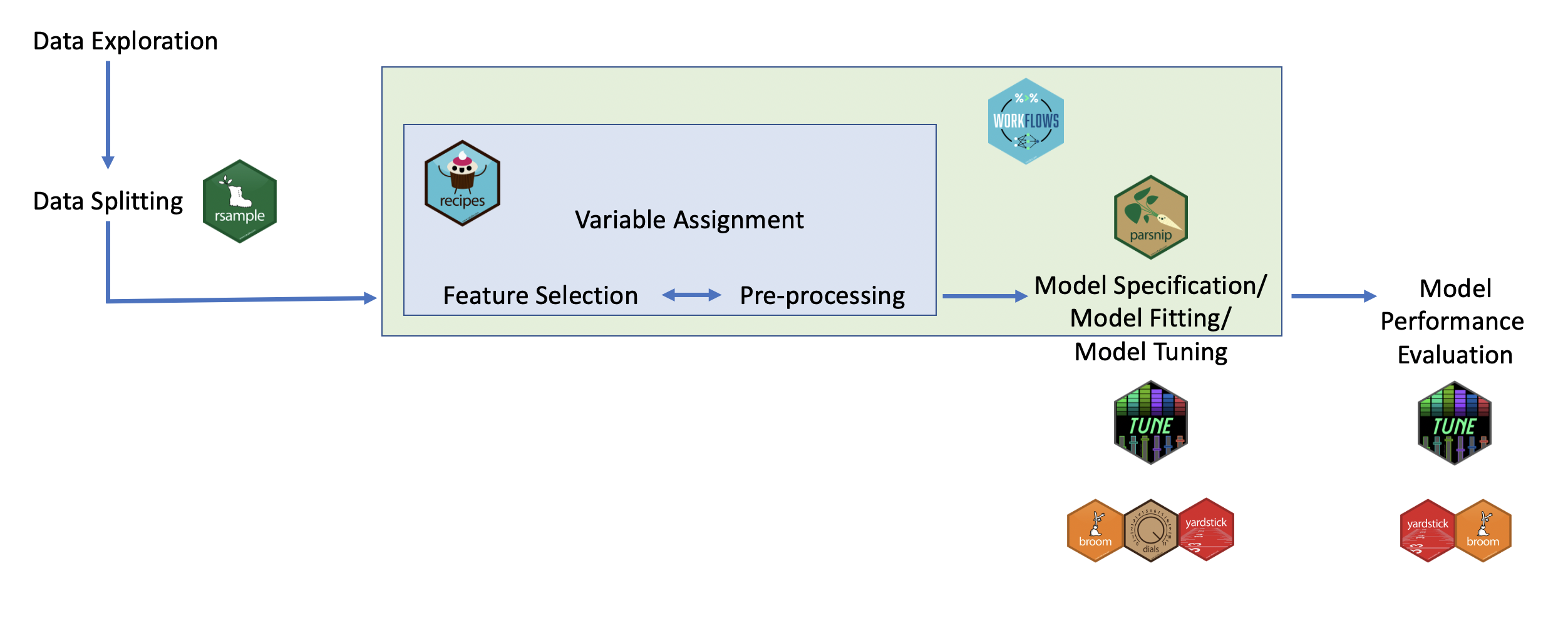
So, the core of the actual ‘machine learning’ happens in the parsnip
package. Before this, you can use the rsample package for splitting
the dataset, and the recipes package for the various preprocessing and
feature selection/engineering steps needed to go from raw data to the
input variables for the machine learning. After model fitting, the
tune package is used to do fine-tuning of the model (hyperparameter
tuning), and yardstick is used to compute the various evaluation
metrics. Finally, the workflows package helps package the
pre-processing and fitting into a single workflow which makes it easier
to use.
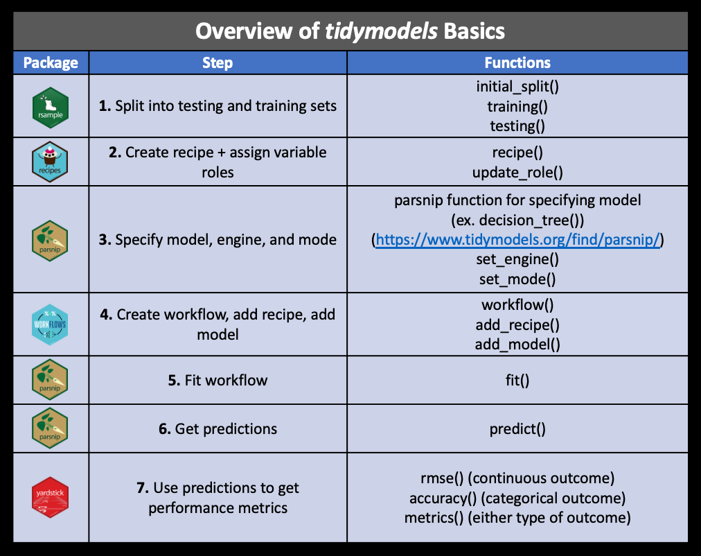
The tutorial below will go through each of these steps. For reference, this figure (from the same source) gives an overview of these packages and key functions:
library(tidymodels)For this tutorial, we will use the ‘german credit data’ dataset:
library(tidyverse)
d <- foreign::read.arff("https://raw.githubusercontent.com/vincentpun123/Credit-Risk-Assessment/refs/heads/main/dataset_31_credit-g.arff")
This dataset contains details about past credit applicants, including why they are applying, checking and saving status, home ownership, etc. The last column contains the outcome variable, namely whether this person is actually a good or bad credit risk.
We can get an overview of all columns using the skimr package: (note
that we also convert all character columns to factor, since they are
represent variables rather than actual text)
d = mutate_if(d, is.character, as.factor)
skimr::skim(d)
To explore relations between variables, you can cross-tabulate e.g. home ownership with credit risk:
table(d$housing, d$class) |>
  prop.table(margin = 1)
So, home owners have a higher chance of being a good credit risk than people who rent or who live without paying (e.g. with family), but the difference is lower than you might expect (74% vs 60%).
We can also make a correlation plot of all numeric variables with the credit score:
d |>
  mutate(class=ifelse(class=='good', 1, 0)) |>
  select_if(is.numeric) |>
  cor(use = "complete.obs") |>
  corrplot::corrplot(diag=F, type = "lower")
So, asking for a longer or higher loan is negatively correlated with being a good credit risk, while being older is a positive correlate.
For an overview of all relations between the outcome and the factor (nominal) predictors, we could plot the distribution of each variable grouped by class:
d |>
  select_if(is.factor) |>
  pivot_longer(-class) |>
  ggplot(aes(y=value, fill=class)) + geom_bar(position='fill') + facet_wrap("name", scales="free", ncol=2)
So, we can see that being a foreign worker or having a deficit on your checking account make you relatively more likely to be a bad credit risk.
Of course, this exploration does not result in a causal interpretation, and in general machine learning does not aspire to yield causal models.
Put bluntly, the goal of the machine learning algorithm is to find out which variables are good indicators of one’s credit risk, and build a model to accurately predict credit risk based on a combination of these variables (called features), regardless of whether they are causally linked with the outcome, or simply proxies or spurious correlates. After all, the bank only cares about whether you will repay the loan, not about why.
Note that this dataset (with only 1000 cases) is pretty small for a machine learning data set. This has the advantage of making it easy to download and the models quick to compute, but prediction accuracy will be relatively poor.
So, after going through the tutorial, you might also want to try to download a larger dataset (and of course you can also do so right away and adapt the examples as needed). A good source for this can be kaggle, which has lots of datasets suitable for machine learning.
The first step in any machine learning venture is to split the data into training data and test (or validation) data, where you need to make sure that the validation (or test) set is never used in the model training or selection process.
We use the initial_split function from rsample, which by defaults
gives a 75%/25% split: (type ?initial_split for more information)
set.seed(123)
split = initial_split(d, strata = class)
train <- training(split)
test <- testing(split)Let’s fit and test a simple naive bayes model.
First, we specify the model that we want to use:
library(discrim)
nb_spec = naive_Bayes(engine="naivebayes")
Note that all tidymodels (parsnip) models have an engine parameter,
which determines the actual packages that will be used to fit the data:
Tidymodels does not actually contain all the various ML algorithms, but
rather presents a unified interface to the underlying packages, like (in
this case) naivebayes. For that reason, the first time you use a
particular engine R will prompt you to install the package:
install.packages("naivebayes")In fact, you can use the translate function to see how the tidymodels
specification is translated to the underlying engine:
nb_spec |> translate()Next, we use this model to fit the training data:
nb_model = fit(nb_spec, class ~ ., data=train)So, how well can this model predict the credit risk? Let’s get the predicted classes for the test set:
predictions = predict(nb_model, new_data=test) |>
  bind_cols(select(test, class)) |>
  rename(predicted=.pred_class, actual=class)
head(predictions)
Since this is just a normal data frame (or tibble), we can compute e.g. the accuracy and confusion matrix using regular R functions:
print(paste("Accuracy:", mean(predictions$predicted == predictions$actual)))
table(predictions$predicted, predictions$actual)
So, on the training set it gets 68% accuracy, which is not very good for
a two-way classification. We can see that the most common error is
mistakenly assigning a good credit score.
Now, we could also write our own code for computing precision, recall, etc., but there are functions built into the yardstick package that make our life a bit easier:
recall(predictions, truth=actual, estimate=predicted)
precision(predictions, truth=actual, estimate=predicted)
The common way to use these is to create a metric set:
metrics = metric_set(accuracy, precision, recall, f_meas)
metrics(predictions, truth = actual, estimate = predicted)
We can see that the model is pretty bad at predicting bad credit risks, with a precision of 46% but a recall of about 35%.
Note that these metrics assume that we are trying to predict ‘bad’
credit risks, since that is the first level of the class factor (levels
are alphabetic by default). We could specify event_level='second' to
make precision and recall relative to ‘good’ credit risks, or specify
estimator='macro' to get the (macro-)averaged f scores
Let’s try another model, this time a support vector machine (SVM). We can specify and fit it just like the Naive Bayes model above:
svm_spec = svm_poly(degree=2, engine="kernlab", mode="classification")
svm_model = fit(svm_spec, class ~ ., data=train)
predictions = predict(svm_model, new_data=test) |>
  bind_cols(select(test, class)) |>
  rename(predicted=.pred_class, actual=class)
metrics(predictions, truth = actual, estimate = predicted)
This already improves the F measure quite a bit, although the result is still far from great.
Properly using SVM, however, introduces two additional layers of
complexity: + Preprocessing: SVM’s require input data to be
centered and scaled (i.e. normalized) as it uses a distance function
to compute the margin: if the dimensions are not on the same scale
(e.g. comparing age in years to income in euros), one dimension will be
much more important in determining this distance. + Parameter
tuning: SVM’s have hyperparameters, or parameters that control the
fitting of the actual model parameters. For all SVM models, there is a
cost parameter that determines the trade-off between misclassification
and wider margins. Kernel based SVM models also have parameters based on
the kernel, for example the polynomial kernel has the degree
hyperparameter.
This allows us to introduce three more useful packages of tidymodels: recipes, workflow and tune.
For SVM, we will center and scale all numeric variables, and create dummies for the factor variables. Finally, we remove any columns with zero variance:
svm_recipe = recipe(class ~ ., data=train) |>
  step_scale(all_numeric_predictors()) |>
  step_center(all_numeric_predictors()) |>
  step_dummy(all_nominal_predictors()) |>
  step_zv(all_predictors())
svm_recipe
We could now prep the recipe to fit it on the training data (so it
knows e.g. which dummies to create), and use it to bake the raw data:
(with apologies for the cullinary metaphors)
prepped = prep(svm_recipe, data=train)
bake(prepped, new_data=train)
As you can see, the numerical values are centered and the factors are turned into dummies.
Rather than doing these steps directly though, it is more convenient to create a workflow that specifies both preprocessing and model fit:
svm_workflow = workflow() |>
  add_recipe(svm_recipe) |>
  add_model(svm_spec)
Note that it would be possible to do this using regular tidyverse commands on the data, and there is no strict need to combine the preprocessing and model fit in a single workflow. The benefit of creating a workflow like this, however, is that it can directly be applied to both training data and testing data. As we will see below, it will also come in handy when doing parameter tuning with crossvalidation.
We can now use the created workflow to directly preprocess and fit the model:
svm_model <- fit(svm_workflow, data = train)
predict(svm_model, new_data=test) |>
  bind_cols(select(test, class)) |>
  rename(predicted=.pred_class, actual=class) |>
  metrics(truth = actual, estimate = predicted)
Embarrassingly, performance actually decreased a tiny bit. As it turns out, the kernlab::kvsm function already does scaling itself, and apparently deals with factors better than creating dummies. Let’s see if we can improve this by doing some parameter tuning!
The SVM model trained above, like many ML algorithms, has a number of (hyper)parameters that need to be set. In this case this includes cost (the tradeoff between increasing the margin and misclassifications) and degree (the polynomial degree).
Although the defaults are generally reasonable, there is no real theoretical reason to choose any value of these parameters. So, the common approach is to test various options and pick the best performing one.
In the section on ‘grid search’ below you will learn the recommended way to do this with a grid search using cross-validation. Before doing that, however, it is instructive to try some different settings ourselves.
First, It is very important here to not use the test set for that, as picking the model based on performance on the test set gives a bias on the accuracy reported by testing on the test set. So, we will split a small set for selecting models from the train set:
result = list()
for (cost in 10^(-1:2)) {
  for (degree in 1:3) {
    result[[paste(cost, degree, sep="_")]] = svm_poly(cost=cost, degree=degree, engine="kernlab", mode="classification") |>
      fit(class ~ ., data=train) |>
      predict(new_data=test) |>
      bind_cols(select(test, class)) |>
      metrics(truth = class, estimate = .pred_class) |>
      add_column(cost=cost, degree=degree)
  }
}
bind_rows(result) |>
  pivot_wider(names_from=.metric, values_from = .estimate) |>
  arrange(-f_meas)
So in this small example, the best result is achieved with a cost of 3d
degree kernel. However, we normally don’t want to write the grid search
ourselves. Moreover, we really shouldn’t be using the test data to do
model selection, as that compromises our estimation of final model
performance. Thus, we will turn to the tune package to do the grid
search.
The package tune is created to make
hyperparameter tuning like above less painful. For this, we change the
model specification to have the degree and cost be tuned:
svm_workflow = workflow() |>
  add_recipe(svm_recipe) |>
  add_model(svm_poly(mode="classification", cost=tune(), degree=tune()))
Next, we define the grid to be searched, specifying 7 levels for the
cost function and 3 for the degree
grid = svm_workflow %>%
  parameters() %>%
  grid_regular(levels=c(cost=7, degree=3))
grid
To tune this, we use crossvalidation:
set.seed(456)
folds <- vfold_cv(train, v = 5)
Now, we are ready to do the grid tuning. Note that this can take a
while, as it will fit and test 3 (degrees) * 5 (folds) * 7 (costs) =
105 models. For this reason, and because with more complex models this
can grow even bigger, we can tell R to run the various models in
parallel using doParallel::registerDoParallel(), so it can take
advantage of multiple processor cores.
doParallel::registerDoParallel()
grid_results = svm_workflow %>%
  tune_grid(resamples = folds, grid = grid, metrics = metrics)
We can gather all results using the collect_metrics, or show the top
results using show_best:
collect_metrics(grid_results)
show_best(grid_results, metric = "f_meas")
From this it seems that a simple model with degree 1 performs best (quite possibly also because of the small data set). The relationship between cost and performance seems less clear, however.
Since collect_metrics returns a regular tibble, we can use normal
tidyverse commands to analyse or visualize it. For example, we can plot
the relation between cost, degree, and f-score:
grid_results %>%
  collect_metrics() %>%
  filter(.metric=="f_meas") |>
  mutate(degree=as.factor(degree)) |>
  ggplot(aes(x=cost, y=mean, color = degree,)) +
  geom_ribbon(aes(
    ymin = mean - std_err,
    ymax = mean + std_err,
    fill=degree
  ),lwd=0, alpha = 0.1) +
  geom_line() +
  scale_x_log10()
So it is important that cost is bigger than about .01, but for the rest it is mostly stable.
To select the best model specification from the grid result
final_svm = grid_results |>
  select_best(metric="f_meas") |>
  finalize_workflow(x=svm_workflow)
And use it to fit on the full training set and test it on the test set:
svm_model <- fit(final_svm, data = train)
predict(svm_model, new_data=test) |>
  bind_cols(select(test, class)) |>
  rename(predicted=.pred_class, actual=class) |>
  metrics(truth = actual, estimate = predicted)
Not unexpectedly, final performance is slightly lower than the performance from the grid search: since we select the model that does best on the cross-validation, it is likely that the model will perform slightly worse out of sample. However, grid tuning did manage to increase our F-score at least a little bit.
Hopefully, this tutorial gave you an idea of how to do machine learning with tidymodels. To get more proficient with this, try using your own data and play around with various ML algorithms and hyperparameters. See the parsnip documentation for a list of possible models.