Replies: 2 comments
-
|
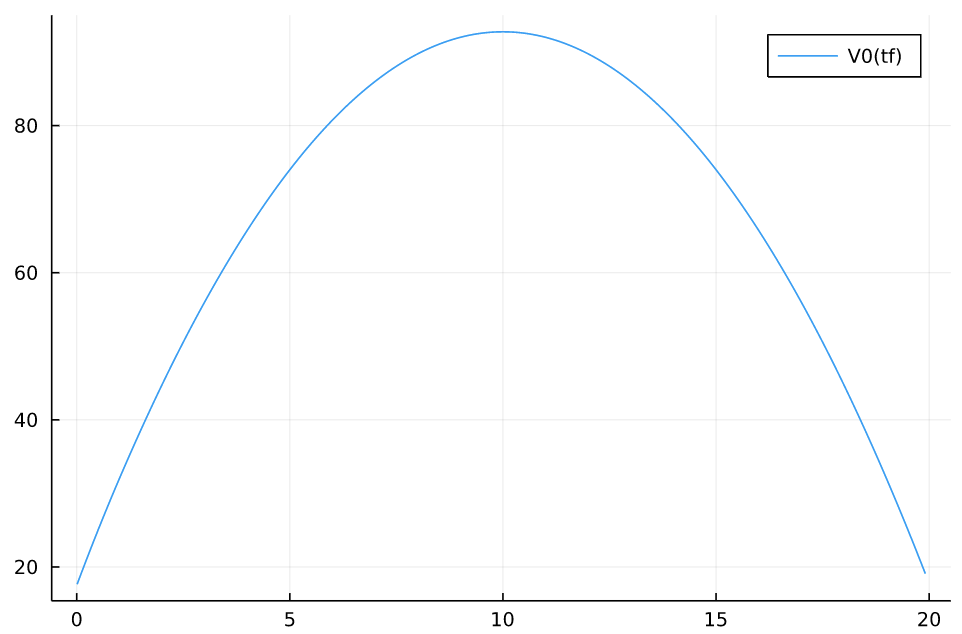
Here is my badly written shooting-method style attempt: function V0(tf)
t0=0.0; #tf=2.0;
u(s,c,t) = s - c;
S(s,t) = s; # s(s(T),T)
LOM1(s,c,t) = -2 + 0.5*c; # ṡ=LOM(s,c)
g1(s,c,t) = c + 0; #
g2(s,c,t) = 1 - c ; #
s_0=17.5;
opt = Ipopt.Optimizer # desired solver
ns = 1_000; # number of points in the time grid
m = InfiniteModel(opt)
@infinite_parameter(m, t ∈ [t0, tf], num_supports = ns)
@variable(m, s, Infinite(t)) ## state variables
@variable(m, c, Infinite(t)) ## control variables
@objective(m, Max, integral(u(s,c,t), t) + S(s(tf),tf))
@constraint(m, LOM_1, deriv(s, t) == LOM1(s,c,t))
@constraint(m, CON_1, g1(s,c,t) >= 0.0)
@constraint(m, CON_2, g2(s,c,t) >= 0.0)
@constraint(m, s(0) == s_0) ## initial condition
optimize!(m)
opt_obj = objective_value(m) # V(B0, 0)
return opt_obj
end
tf_grid = 0.01:0.1:20.0
V0_grid = [ V0(ttf) for ttf in tf_grid]
plot(tf_grid, V0_grid)
tf_grid[argmax(V0_grid)]Now solve using the optimal T* if 1==1
t0=0.0; #
tf=tf_grid[argmax(V0_grid)];
u(s,c,t) = s - c;
S(s,t) = s; # s(s(T),T)
LOM1(s,c,t) = -2 + 0.5*c; # ṡ=LOM(s,c)
g1(s,c,t) = c + 0; #
g2(s,c,t) = 1 - c ; #
s_0=17.5;
opt = Ipopt.Optimizer # desired solver
ns = 1_000; # number of points in the time grid
m = InfiniteModel(opt)
@infinite_parameter(m, t ∈ [t0, tf], num_supports = ns)
@variable(m, s, Infinite(t)) ## state variables
@variable(m, c, Infinite(t)) ## control variables
@objective(m, Max, integral(u(s,c,t), t) + S(s(tf),tf))
@constraint(m, LOM_1, deriv(s, t) == LOM1(s,c,t))
@constraint(m, CON_1, g1(s,c,t) >= 0.0)
@constraint(m, CON_2, g2(s,c,t) >= 0.0)
@constraint(m, s(0) == s_0) ## initial condition
optimize!(m)
termination_status(m)
c_opt = value(c)
s_opt = value(s)
ts = supports(t)
opt_obj = objective_value(m) # V(B0, 0)
# using Plots
ix = 2:(length(ts)-1) # index for plotting
plot(legend=:topright)
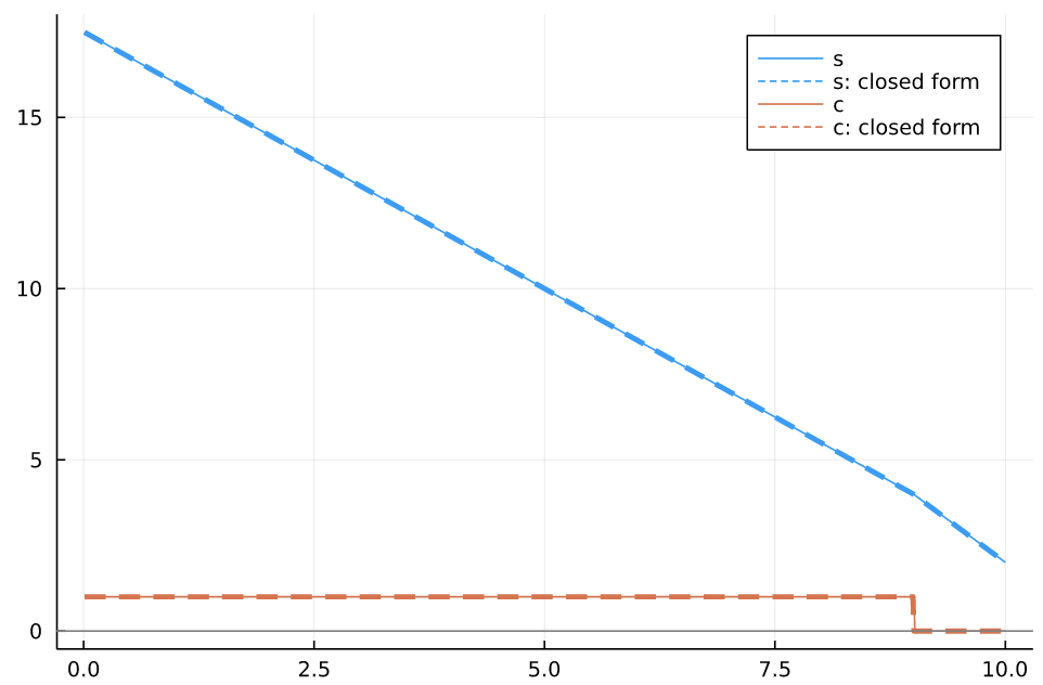
plot!(ts[ix], s_opt[ix], c=1, lab = "s")
plot!(ts[ix], tt -> tt<9 ? 17.5 -1.5tt : 22-2*tt , c=1, l=:dash, lw=3, lab = "s: closed form")
plot!(ts[ix], c_opt[ix], c=2, lab = "c")
plot!(ts[ix], tt -> tt<9 ? 1 : 0, c=2, l=:dash, lw=3, lab = "c: closed form")
plot!([0.0], seriestype = :hline, lab="", color="grey")
end
I bet there are MUCH better/faster ways to implement this. PS: here is a plot of |
Beta Was this translation helpful? Give feedback.
-
|
Hi there again. Indeed, rather than a grid search, we can directly pose this as an optimization problem via reformulation. The key idea is to replace the infinite parameter t (time) with an infinite parameter that indexes progress (from 0 to 1) toward some sort of termination condition. This is explained quite well in the video tutorial at https://apmonitor.com/wiki/index.php/Apps/RocketLaunch. So for your problem, let's use a progress parameter using InfiniteOpt, Ipopt
m = InfiniteModel(Ipopt.Optimizer)
@infinite_parameter(m, τ ∈ [0, 1], num_supports = 1000)
@variable(m, s, Infinite(τ)) # state variable
@variable(m, 0 ≤ c ≤ 1, Infinite(τ)) # control variable
@variable(m, 5 ≤ tf ≤ 15, start = 12) # final time (bounds help with convergence but are optional)
@objective(m, Max, tf * ∫(s - c, τ) + s(1)) # note that we need to scale the integral by tf
@constraint(m, LOM_1, ∂(s, τ) == tf * (-2 + 0.5 * c)) # scale the equation by tf
@constraint(m, s(0) == 17.5) ## initial condition
optimize!(m)
ts = value(τ) * value(tf) # scaled times
u_opt = value(u)
c_opt = value(c)With this I get |
Beta Was this translation helpful? Give feedback.
Uh oh!
There was an error while loading. Please reload this page.
-
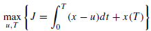
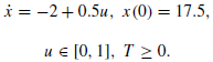
I've seen some discussions about free terminal time problems, but don't know how to implement it on this simple textbook problem:
The closed form solution:

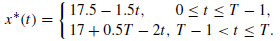

Where control:
Beta Was this translation helpful? Give feedback.
All reactions