Exercises_Lecture03.md

Train a Perceptron!

Introduction

Ok, finally we'll actually train a machine learning system!!

The goal is to separata data like this

def generate_data(N):
    s1 = np.random.multivariate_normal([1,1],[[1,0],[0,1]], size = N)
    s2 = np.random.multivariate_normal([-1.5,-1.5],[[1,0.2],[0.2,1.0]], size = N)
    X = np.concatenate([s1,s2])
    z = np.concatenate([np.ones(N),np.zeros(N)])
    return X,z

X,z = generate_data(200)
plt.scatter(X[:,0],X[:,1],c = z)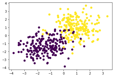

Setting up Variational Inference

We assume the data is produced from a conditional model $p(x|z)$ and we want to find the posterior $p(z|x)$. As an approximation we use the parametrized density

$$ q(z|\theta) = \mathrm{Bernoulli(z|\theta}) = \begin{cases} \theta & \mathrm{for} & z = 1 \\ 1-\theta & \mathrm{for} & z = 0\end{cases} $$

Following the "amortized variational inference" approach, we assume that we can approximate $p(z|x)$ by learning a data-dependent function $\theta(x)$.

The plan is to train a "soft" percepton as discussed in the lecture

$$ \theta_{\vec{w},b}(x) = \sigma(w \cdot x + b) $$

such that $p(z|x) \approx q(z|x) = \mathrm{Bernoulli(z|\theta(x)})$

We will break this down into three function and combine all parameters into a single parameter vector

$$ \phi = (w_1,w_2,b) $$

1. First the linear mapping: $h(x) = \vec{w} x + b$ mapping $h: \mathbb{R}^2 \to \mathbb{R}$

   def linear(x,parameters):
       out = x @ parameters[:2].T + parameters[2]
       return out

2. Second, the squashing function $\sigma: \mathbb{R} \to [0,1]$

   def sigmoid(x):
       out = 1/(1+np.exp(-x))
       return out

3. Third, the loss function $l(z,\theta) = -\log q(z_i|\theta)$

   def loss(z, theta):
       out = np.where(z==1,-np.log(theta),-np.log(1-theta))
       return out

In order to estimate the loss for the full dataset, we need to compute the empirical risk $\hat{L} = -\sum_{z_i,x_i} \log(z_i | \theta(x_i))$

def empirical_risk(X,z,pars):
    mapped = linear(X,pars)
    theta = sigmoid(mapped)
    loss_val = loss(z,theta)
    return loss_val.mean(axis=0)

We can can plot the decision function $\theta(x)$ on the plance $(x_1,x_1) \in \mathbb{R}^2$ using a function like this

def plot(X,z,pars):
    grid = np.mgrid[-5:5:101j,-5:5:101j]
    Xi = np.swapaxes(grid,0,-1).reshape(-1,2)   
    p = sigmoid(linear(X,pars))
    zi = sigmoid(linear(Xi,pars))
    zi = zi.reshape(101,101).T
    plt.contour(grid[0],grid[1],zi)
    plt.scatter(X[:,0],X[:,1],c = z)
    plt.xlim(-5,5)
    plt.ylim(-5,5)

Step 1 Plot a fixed Percepton

Use the above functions to plot the percepton and the data for a fixed parameter vector $\phi = (2.0,-1.0,0.0)$

Gradient Calculation

In order to train the perceptron we need to have the empirical risk value and its derivative

$$\hat{L}, \frac{\partial \hat{L}}{\partial \phi}$$

Using the definitions we get

$$ \frac{\partial \hat{L}}{\partial \phi} = \sum_i \frac{\partial}{\partial \phi}l(z_i,\sigma(h(x)) $$

That is, if we just need to find an expression for $\frac{\partial}{\partial \phi}l(z_i,\sigma(h(x))$. By the chain rule

$$ \frac{\partial}{\partial \phi}l(z_i,\sigma(h(x)) = \frac{\partial l}{\partial \sigma} \frac{\partial \sigma}{\partial h} \frac{\partial h}{\partial \phi} $$

Step 2

Derive an expression for the the derivative $\frac{\partial h}{\partial \phi}$

Step 3

Show that the derivative of $\sigma(x)$ corresponds to

$$ \sigma'(x) = \sigma(x)(1-\sigma(x)) $$

Step 4

Derive the derivative of $\frac{\partial l(z,\theta)}{\partial \theta}$ for both $z=0$ and $z=1$

Step 5

Adapt the functions linear(..), sigmoid(...), loss(...) such that they return

1. The function value
2. The gradient value at the point at which the function was evaluated

def function(...)
    out = ...
    grad = ...
    return out,grad

Hint: as we will evluate the function on many inputs at the same time make sure to return a "column" vector of shape (N,1) for the sigmoid and loss functions

Step 6

Using the chain rule and the individual gradient computations, adapt empirical_risk similarly to return

1. $\hat{L}$
2. $\frac{\partial \hat{L}}{\partial \phi}$

Step 7

Write a Training Loop!

1. Initialize the parameters with $\phi = (1.0,0.0,0.0)$
2. Allow 2000 iterations of improving the parameters
3. For each iteration update the parameters with Gradient Descent and a Learning Rate of $\lambda=0.01$

$$ \phi \leftarrow = \phi - \lambda \frac{\partial \hat{L}}{\partial \phi}$$

4. After every 500 steps, plot the current configuration using plot(...) (Note: now that the functions return multiple return values, the plot function needs to be adapted a bit

Step 8

Congratulations, you wrote your first full ML loop!. You can now play with the details of generate_data to try out a few data configurations and convince yourself that your algorithm will find a good decision boundary every time.