Let's denote a commitment to a value v as C = Comm(v). The recipient cannot infer any information about v given C (property called hiding) and cannot find v1 which is different from v and Comm(v1) = C (this means the prover cannot change her mind later, the property is called binding).
Commitment can be thought of as an envelope - the value is put in the envelope and sealed. Upon receiving a commitment, a verifier cannot tell what is inside (hiding) and the prover cannot sneak another value in the envelope later (binding).
A commitment can be later open to reveal what is inside.
Commitment schemes have many applications. Consider for example Alice and Bob flipping the coin and communicating over the phone (they are not in the same place). Instead of reporting the actual coin flip, Alice only tells Bob a commitment of the value. Bob then flips the coin and reports the result. Alice now reveals what she commited to (Bob cannot cheat).
For commitments schemes the following two properties need to hold (informally):
- secrecy (hiding): (almost) no information is revealed to the verifier
- unambiguity (binding): your chances of being able to change your mind are very small (the sender cannot change the message)
There is a special subset of commitment schemes called trapdoor commitment schemes. Trapdoor commitment schemes allows to overcome the binding property if you know a special information (called trapdoor). This means that a committer can change her mind and open a commitment abiguously.
We will see below how trapdoor commitment schemes can be used to build zero knowledge proofs out of sigma protocols. Note: it is much easier to prove that a protocol is a sigma protocol than to prove that a protocol is a zero knowledge proof of knowledge.
Receiver chooses:
- large primes p and q such that q | p-1.
- generator g of order q subgroup of Z_p*
- random secret a from Z_q
- h = g^a % p
Values p, q, g, h are public, a is secret (a is called trapdoor).
When committing to some x from Z_q, sender chooses random r from Z_q and sends c = (g^x * h^r) % p to receiver.
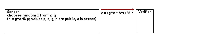
When a sender reveals x and r, receiver verifies that c = (g^x * h^r) % p.

Note that Pedersen commitment is a trapdoor commitment scheme: if the committer knows the exponent a (trapdoor), she can decommit c to an arbitrary value x'. Decommitter simply reveals (x', r' = r + (x - x')/a). It holds:
(g^x' * h^r') % p = (g^x' * h^r * h^((x-x')/a)) % p = (g^x' * h^r * g^(x-x')) % p = g^x * h^r = c
Verifier V generates safe primes P and Q: P = 2p +1, Q = 2q + 1 where p, q are different primes. V then find at random g_p of order p in G_p and g_q or order q in G_q, where G_p, G_q are subgroups of order p,q in Z_P*, Z_Q* respectively. V then computes b_0 via CRT:
b_0 = g_p mod P
b_0 = g_q mod Q
Note that b_0 is generator of G_(p*q).
V generates random alpha from Z_(p*q)* and sets b_1 = b_0^alpha mod N.
Commitment is:
BC(x, r) = b_0^x * b_1^r mod N where x < N and r < 2^m * N where k is security parameter.
Miller's lemma [14]: Let's N = p * q and lambda(N) = (p-1) * (q-1) (the Carmichael function). On input (N, L) where L is a multiple of lambda(N), N can be factorized with non-negligible probability. Note that lambda(N) = (p-1) * (q-1).
Let's say we can can find (r1, s1) and (r2, s2) such that:
b_0^s1 * b_1^r1 = b_0^s2 * b_1^r2 mod N
b_0^(s1 - s2) * b_1^(r1 - r2) = 1 mod N
Thus, we are able to find (r, s) such that:
b_0^s * b_1^r = 1 mod N
b_0^(s + alpha * r) = 1 mod N
The order of b_0 is pq, thus pq | (s + alpha * r). In our case lambda(N) = (P - 1) * (Q - 1) = 4 * p * q. If we take 4*(s + alpha * r), we have L from Miller's lemma and we can factorize N.
Zero-knowledge proof is an interactive proof where verifier learns nothing beyond the correctness of the statement being proved. Zero-knowledge proofs can be used to enforce the proper behavior of the verifier.
Zero-knowledge proofs have been introduced in the seminal paper of Goldwasser, Micali, and Rackoff [5].
Before [5] interactive proof systems mostly considered the cases where a malicious prover attempts to convince a verifier to believe a false statement. In [5] also the verifier was considered as someone who can cheat. The authors asked if the verifier can be convinced about a statement without any information being leaked except for the validity of the statement.
The majority of the notes below are taken from Hazay-Lindell [1] Sigma protocols and efficient zero-knowledge chapter which is based on [2].
Many zero-knowledge protocols are constructed from a simpler primitive called sigma protocol (it is far easier to construct a protocol and prove that it is a sigma protocol, than to construct a protocol and prove that it is zero-knowledge proof of knowledge).
In the interactive proof the prover wants to ascertain a verifier whether a given string belongs or not to a formal language. The prover posseses unlimited computational resources, but cannot be trusted. The verifier has limited computation power.
For the interactive proof two requirements need to hold:
- completeness: if the string belongs to a language, the honest verifier (the one that follows the protocol properly) can be convinced of this fact by untrusted prover
- soundness: if the string does not belong to the language, no prover can convince the honest verifier that it belongs, except with some small probability
Zero knowledge proof is an interactive proof with the additional property that the verifier learns nothing but the correctness of the statement (that the string belongs to the language).
A simple example of a zero knowledge proof is the proof of knowledge of a discrete logarithm. This can be done by Schnorr's protocol:
- prover wants to prove that t = g^s % p
- system parameters are large primes p and q such that q | p-1; g is a generator of a subgroup of order q in Z_p* (subgroup is Schnorr group, see number_theory.md)
- prover chooses random r from Z_q and sends x = g^r % p to verifier
- verifier knows t and wants a proof that prover knows its discrete logarithm (t can be thought as a public key, while s is a secret key)
- verifier chooses random c from [1,...,2^n] and sends it to a prover (n is fixed such that 2^n < q)
- prover sends y = (r+s*c) % q to the verifier
- verifier verifies that g^y = g^r * (g^s)^c (mod p)

Note that a verifier cannot extract s from y = r + s*c since she does not know r (to extract r a discrete logarithm would need to be solved). Also note that if c is not chosen randomly (if prover can predict the value c), the prover can set x = g^y * t^(-c) and convince the verifier that she knows the secret witout really knowing it.
At the end of the Schnorr's identification protocol the verifier is convinced he is interacting with the prover, or better to say - with someone who knows the secret key that corresponds to the prover's public key. Which means with someone who knows the dlog of t.
Schnorr's protocol can be used as identification protocol and is different from the standard password authentication where prover's secret key is her password pw and public key is hash(pw). Here the prover sends hash(pw) and the verifier checks whether this matches the stored value. However this is not secure agains eavesdropping attacks as the adversary who observes one interaction between prover and verifier and sees hash(pw), can later impersonate a prover.
The required properties for zero knowledge proofs are:
- completeness: if the statement is true, the honest verifier (the verifier that follows the protocol properly) will be convinced of this fact with overwhelming probability
- soundness: no one who does not know the secret can convince the verifier with non-negligible probability
- zero knowledge: the proof does not leak any information
Zero knowledge property is usually demonstrated with an existance of a simulator that produces a fake transcript of protocol messages that is indistinguishable from the actual protocol messages. If all messages can be thus simulated, verifier does not learn anything new during the protocol.
There is also a notion of honest-verifier zero knowledge protocol which means that the protocol is zero knowledge if the verifier follows the protocol honestly.
Why is the size of challenge (t) important - because if the prover can guess the challenge, she chooses z and sets the first message as g^z * h^(-e) - and thus convince the verifier.
Soundness can be demonstrated by an existance of a knowledge extractor algorithm which can extract the secret from a prover. The intuition behind is - if a prover can convince the verifier that she knows the secret without actually knowing it, then no algorithm could extract the secret from a prover.
The Schnorr's protocol is sound because there exists an algorithm which extracts a secret from a prover if prover is used as a black-box.
If the protocol is executed two times and prover is rewinded between the two executions so that it sends the same first message, then if both executions were sucessful (y1 and y2 sent by a prover in the last step were verified), the algorithm can compute the secret.
The algorithm (extractor) has c1, c2 and y1, y2:
g^y1 = g^r * (g^s)^c1
g^y2 = g^r * (g^s)^c2
It holds:
g^(y1-y2) = g^(s*(c1-c2))
And thus:
s = (y1-y2) * (c1-c2)_inv
Note that the prover might use some trick with y1 and y2 to convince the verifier that it knows the secret, however the reasoning above shows that the prover actually knows the secret if it is able to succesffully run the protocol two times.
Schnorr's protocol is honest-verifier zero knowledge (below more about this), it is not known if it is zero knowledge.
Zero-knowledge property can be shown by the existance of a simulator with which we can simulate acceptable protocol runs without knowing the actual language statement.
This can be done for Schnorr protocol if there are no many possible challenges c. Here again, a rewinding technique is used. We choose y1, try to guess c1, compute x1 = g^y1 * t^(-c1). If we now send x1 to the verifier and get c1 (for which there is a high probability, because the space for challenges is small), the transcript (x1, c1, y1) will be accepted. If we didn't correctly guess c1, we rewind to the beginning. That means we provide a new x1 (now we know the challenge c1) and send a new x1 to the verifier. Verifier will respond with the same challenge c1 (rewinding).
Thus Schnorr protocol is perfect zero-knowledge when the challenge space is small. But if the challenge space is small, the prover needs to run the protocol many times to convince the verifier. However it can be proved that it is honest-verifier zero-knowledge for when the challenge space is large. When verifier is honest, the challenges c are chosen randomly and the simulator can be pretty much the same as above, but we let the simulator choose random c (no need for guessing).
So, we can simulate acceptable runs without knowing s (s is secret, we know only t = g^s % p). If the verifier is dishonest he could (instead of choosing a random challenge) choose a challenge c based for example on the input x and there is no known simulator which could simulate such transcripts. Schnorr protocol is thus honest-verifier zero-knowledge. But it can be made a fully zero-knowledge by using commitment scheme.
We don't know whether Schnorr protocol is zero-knowledge (whether verifier could extract some information about s after having a number of transcripts). However, a description how to make sigma protocols by using commitment scheme to be zero-knowledge is given below.
Schnorr signature is obtained by applying the Fiat-Shamir transformation to the Schnorr protocol.
The setup of parameters is as in Schnorr id scheme described above. The difference is that instead of challenge c being chosen by a verifier, prover calculates c = hash(m || g^r), where m is a message that is to be signed. The signature is then (y, c), where y = r + s*c
Verifier needs to check g^y = g^r * (g^s)^hash(m || x) (mod p).

Let R be a binary relation, where the only restriction is that if (x, w) is from R, then the length of w is at most p(|x|) for some polynomial p(). We may think of x as an instance of some computational problem. For example for discrete log problem we can define relation:
R_DL = {((G, q, g, h), w); h = g^w}
where G is group of order q with generater g, q is prime, and w is from Z_q. R_DL contains the entire set of discrete log problems with their solutions.
We consider the protocols of the following form:
- Common input: the prover P and verifier V both have x.
- Private input: P has a value w such that (x, w) is from R.
- The protocol template:
- P sends V a message a.
- V sends P a random t-bit string e.
- P sends a reply z, and V decides to accept or reject based solely on the data it has seen (based on value x, a, e, z).
A transcript (a, e, z) is an accepting transcript for x if the protocol instructs V to accept based on the value (x, a, e, z).
A protocol is sigma protocol for relation R if it is a three-round public-coin protocol of the form above and the following requirements hold:
- Completeness: If P and V follow the protocol on input x and private input w to P where (x, w) from R, then V always accepts.
- Special soundness: There exists a polynomial-time algorithm A that given any x and any pair of accepting transcripts (a, e, z), (a, e', z') for x, where e!=e', outputs w such that (x, w) from R.
- Special honest verifier zero knowledge: there exists a probabilistic polynomial-time simulator M, which on input x and e outputs a transcript of the form (a, e, z) with the same probability distribution as transcripts between the honest P and V on common input x.
It is clear that Schnorr's protocol is sigma protocol - the simulator for special soundness is described above (you have two transcripts (a, e, z) and (a, e', z'), so you have g^z = g^r * g^(e * w) and g^z' = g^r * g^(e' * w), from where you get g^((z-z')/(e-e')) = g^w and you have w). The simulator for special honest verifier zero knowledge is: you take random z and random e, compute a = g^z * h^(-e) (you don't need to know w) and you have a transcript which has exactly the same probability distribution as a real conversation between the honest prover and honest verifier. However there are many other examples of sigma protocols.
Note that sigma protocol also proves that x has a solution (in dlog there is always a solution, but in other cases this is not necessary) with probability > 1-2^(-t). This is because if the solution w does not exist, there exists for every a at most one query e that results in an accepting transcript (otherwise w would be obtained due to special soundness property and thus the solution of x would exist), so the prover would convince the verifier with the probability at most 2^(-t).
Given a tuple (G, q, g, h, u, v) can we prove that there exists w such that u = g^w and v = h^w? Let's define a protocol:
- P and V both have (G, q, g, h, u, v)
- P has a value w such that u = g^w and v = h^w
The protocol:
- P chooses a random r from Z_q, computs a = g^r and b = h^r and sends (a, b) to V.
- V chooses a random challenge e from {0,1}^t where 2^t < q and sends it to P.
- P sends z = r + e * w mod q to V, which checks that g^z = a * u^e and h^z = b * v^e, that G is a group of order q wither generators g and h, and that u, v are from G.
If we show that this is sigma protocol, we have a way to prove that there exists w such that u = g^w and v = h^w. The completeness holds because (similarly for h^z = b * v^e):
g^z = g^(r + e * w) = g^r * g^(w * e) = g^r * (g^w)^e = a * u^e
Special soundness: for two transcripts ((a, b), e, z) and ((a, b), e', z') we get w as for the Schnorr's protocol from either of the two equations: g^(z-z') = u^(e-e') and h^(z-z') = v^(e-e').
The special honest verifier zero knowledge property can be shown as for the Schnorr's protocol.
If you execute sigma protocol in paralell l-times, the resulting protocol is a new sigma protocol with challenge length l * t.
Note that the probability that a prover guesses a challenge is 2^(-t) for one execution, if there are l executions, the probability is 2^(-l * t). Thus, the soundness error is reduced to 2^(-l * t).
If there exists a sigma protocol SP1 for R with challenge length t, then there exists a sigma protocol SP2 for R with challenge length t', for any t'.
If t' is smaller than t, we define a new sigma protocol SP2 as follows - SP2 sends the first message as in SP1. V sends a random t'-bit string e. In the last step SP2 appends t-t' 0s to e and use this value to compute the message z. V then checks z as in SP1. Completeness and special soundness obviously still holds. Special zero knowledge holds because the simulator M (which exists for SP1) works for every challenge e (it generates an accepting transcript out of e).
If t' is bigger than t, the SP2 can be constructed by running SP1 in parallel multiple times and then adjust the length down (as above) to t' if needed.
We haven't proved that sigma protocol is really a proof of knowledge yet. Intuitively, the special soundness is equivalent to the proof of knowledge, however, the proof should say how the two accepting transcripts are found.
The standard definition of proofs of knowledge which is given below was proposed by Bellare and Goldreich [4]. Roughly, some older definitions went like this: if the verifier is always convinced, then there exists a knowledge extractor which can extract a knowledge from a prover. Bellare and Goldreich proposed definition which takes into account cases when the prover is able to convince the verifier with some non-constant probability smaller than 1.
Let's first formally define what is a proof of knowledge. Let kappa: {0, 1}* -> [0, 1] be a function. A protocol (P, V) is a proof of knowledge for the relation R with knowledge error kappa if the following two properties are satisfied:
-
Completeness: If P and V follow the protocol on input x and private w to P where (x, w) from R, then V always accepts.
-
Knowledge soundness (or validity): There exists a constant c > 0 and a probabilistic oracle machine K (knowlege extractor) such that for every interactive prover function P* and every x from L_R (L_R are all x for which a solution w exists), the machine K satisfies the following condition. Let epsilon(x) be the probability that V accepts on input x after interacting with P*. If epsilon(x) > kappa(x), then upon input x and oracle access to P*, the machine K outputs w such that (x, w) is from R within an expected number of steps bounded by:
|x|^c/(epsilon(x) - kappa(x))
If SP is a sigma protocol for a relation R with challenge length t, then SP is a proof of knowledge with knowledge error 2^(-t).
Completeness holds by definition. What we need to show is that we are able to find two accepting transcripts "sufficently" quickly. Let's visualize all possible interactions in a matrix - one row for each possible choices by P, one column for each possible challenge value e.
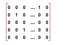
I assume by this is meant that each row presents a possible first message in a protocol. The matrix contains 1 if P can convince V for the first message (which defines this row) and for the challenge that defines this column (there are 2^t possible values for challenge), otherwise there is 0. The goal is to find two 1's in one row - when this is done, the special soundness gives as the result.
epsilon(x) is the probability that V is convinced (for each x there is its own matrix)- epsilon(x) is the fraction of 1's in the matrix, but this does not say anything about how 1's are distributed in rows. If we start searching in a row where there is only a single 1, we have to break at some point and start looking in other rows (but we don't know if we are in a row like this).
It turns out we can design an algorithm which will find two 1's in a row "sufficiently" quickly.
It is obvious how to construct a sigma protocol to prove an AND statement. Simply, the prover proves both statements in parallel - the verifier sends a single challenge for both proofs.
For OR statements the construction is more complex. Both, P and V, have a pair (x_0, x_1). P wants to prove to V that it knows w such that either (x_0, w) from R_0 or (x_1, w) from R_1 (w is solution for either x_0 or x_1).
Let b be such that (x_b, w) is from R_b. The protocol goes like this:
-
P computes the first message a_b using (x_b, w) as input. P chooses e_(1-b) at random and runs the simulator M on input (x_(1-b), e_(1-b)) - let (a_(1-b), e_(1-b), z_(1-b) be the output of M. P sends (a_0, a_1) to V.
-
V chooses a random t-bit string s and sends it to P.
-
P sets e_b = s xor e_(1-b) and computes the answer z_b to challenge e_b (the other z is from the output of M). P sends (e_0, z_0, e_1, z_1) to V.
-
V checks that e_0 xor e_1 = sand that both transcripts are accepting.
As we saw above sigma protocol is a proof of knowledge. However, it is not a zero knolwedge proof of knowledge - because it requires an honest verifier.
The problem is that the challenge generation of the verifier cannot be simulated. Note that the point of zero knowledge proof is that the verifier learns nothing about the statement (except that it is correct), so if the verifier cheats and doesn't follow the protocol properly, it might be able to somehow extract some knowledge (instead of choosing a challenge randomly, the verifier could choose it somehow based on the first message). For this reason we have to be somehow assured that verifier does not cheat.
This can be solved by having the verifier commit to its challenge e before the execution begins (this way the verifier cannot choose some special e once he knows the first message a). The protocol then goes:
- V chooses a random t-bit string e and interacts with P via the commitment protocol in order to commit to e.
- P computes the first message a and sends it to V.
- V decommits to e to P.
- P verifies the decommitment and aborts if it is not valid. Otherwise, it computes the answer z and sends it to V.
- V accepts if and only if transcript is accepting.
If a commitment scheme is perfectly-hiding (because the prover is assumed infinitely powerful, whereas the verifier is restricted to be a probabilistically polynomial time and thus computationally binding scheme suffices), then the sigma protocol extended as above is a zero knowledge proof for L_R with soundness error 2^(-t).
The complexity of the protocol above depends on the cost of running a perfectly-hiding commitment protocol. One possibility is to use Pedersen commitment protocol (see Commitment schemes section above) which is highly efficient.
However, the zero knowledge protocol above is not a proof of knowledge. The problem is that extractor cannot send prover two different e != e' for the same a, because it is committed to e which was sent in the first step.
Let's extend the protocol in the following way (we need a perfectly-hiding trapdoor commitment scheme):
- V chooses a random t-bit string e and interacts with P via the commitment protocol in order to commit to e.
- P computes the first message a and sends it to V.
- V decommits to e to P.
- P verifies the decommitment and aborts if it is not valid. If valid, it computes the answer z. It sends z and trapdoor to V (verifier cannot use trapdoor to cheat anymore, because he already decommitted) .
- V accepts if and only if the trapdoor is valid and the transcript is accepting.
The difference is that now the extractor can obtain the trapdoor and get e' != e (using trapdoor) for the same a.
It can be proved that this protocol is zero-knowledge proof of knowledge.

Note that Pedersen commitment is a trapdoor commitment scheme (see the first section on this page) and can be thus used to construct a zero-knowledge proof of knowledge.
But before zero-knowledge proofs briefly about Boolean circuits and one-way functions
Boolean circuit is a generalization of Boolean formulae and a formalization of a silicon chip. Boolean circuit is a digram showing how to derive an output from an input by a combination of the basic Boolean operations of OR, AND, and NOT. Boolean circuit is called a Boolean formula if each node has at most one outgoing edge.
It can be shown that Boolean circuits implements functions from {0, 1}^n to {0, 1}^m. Boolean operations OR, AND, and NOT form a universal basis, meaning that every function from {0,1}^n to {0,1}^m can be implemented by a Boolean circuit (actually, a Boolean formulae).
A silicon chip is an implementation of a Boolean circuit using a technology called VLSI. If we have a small circuit for a computational task, it can be implemented very efficiently as a silicon chip.
Boolean circuits are a natural model for nonuniform computation where different algorithms are allowed for each input size. On the other hand, in uniform computation the same Turing machine solves the problem for inputs of all sizes.
Most of the cryptography is based on one-way functions - functions that are easy to evaluate but hard to invert.
Definition: A function f:{0,1}* -> {0,1}* is called one-way if the following the conditions hold:
- easy to evaluate: there exist a polynomial-time algorithm A such that A(x) = f(x) for every x from {0,1}*
- hard to invert: for every family of polynomial-size circuits {C_n}, every polynomial p, and all sufficiently large n,
Pr[C_n(f(x)) from f^(-1)(f(x))] < 1/p(n), where the probability is taken uniformly over all the possible choices of x from {0,1}^n.
Vadhan's A study of statistical zero knowledge proofs [10] gives some good introduction into the topic.
To facilitate a complexity-theoretic study of ZKPs, assertions are thought as strings written in some fixed alphabet, and their interpretations are given by a language L identifying the valid assertions. For example, assertions about 3-colorability of graphs can be formalizaed we can talk about a string x as a graph and the language L being the set of x which are 3-colorable. Assertion is then x ϵ L which means x is 3-colorable. The language L is defining the decision problem: given a string x, decide whether it is in L or not. Thus, "assertion", "language", "problem" are often used interchangeably in informal discussions.
The complexity class NP consists of the languages possessing efficiently verifiable proofs. A language L is in NP if there exists an efficient proof-verification algorithm (verifier) satisfying:
- completeness: for every valid assertion (every string in L), there exists a proof that the verifier will accept
- soundness: for every invalid assertion (everyt string not in L), no proof can make the verifier accept
Efficient means that the verifier should run in time polynomial in the length of the assertion (written as a string).
Interactive proofs introduced by [5] serve the same purpose as the above "classical" proofs - to convince a verifier with limited computation power that some assertion is true. However, this is no longer accomplished by giving the verifier a fixed, written proof, but rather by having the verifier to interact with a prover that has unbounded computation power. The verifier's computation time is still polynomial in the length of the assertion, but now both the prover and verifier may be randomized. Such a proof is a randomized and dynamic process that consists of tricky questions asked by the verifier, to which the prover has to reply convincingly.
The notion of completeness and soundness in interactive proof is now slightly relaxed (see "high probability"):
- for every valid assertion, there is a prover strategy that will make the verifier accept with high probablity
- for every invalid assertion, the verifier will reject with high probability, no matter what strategy the prover follows
The complexity class IP is the class of languages possessing interactive proofs. Clearly, every language that possesses a classical proof also possesses an interactive proof (the prover simply sends the classical proof). It has been shown that many more languages possess interactive proofs than classical ones (IP is much larger than NP).
A zero-knowledge proof is an interactive proof in which the verifier learns nothing from the interaction with the prover, other than the assertion being proven is true. This is guaranteed by requiring that whatever the verifier sees in the interaction with the prover is something it could have efficiently generated on its own. That means a polynomial-time simulator should exist that simulates the verifier's view of the interaction of the prover. As the interaction between the prover and verifier is probabilistic, the simulator is also probabilistic, and it is required that it generates an output distribution that is "close" to what the verifier sees when interacting with the prover. Intuitively, this means that the verifier learns nothing because it can run the simulator instead of interacting with the prover.
In [5] three different interpretations of "close" were suggested:
- perferct zero knowledge: requires that the distributions are identical
- statistical zero knowledge: requires that the distributions are statistically close
- computational zero knowledge: requires that the distributions cannot be distinguished by any polynomial-time algorithm
PKZ, SZK, and CZK are the classes of languages possessing perfect, statistical, and computational zero-knowledge proofs.
Pefect and statistical zero knowledge means that the zero-knowledge condition is meaningful regardless of the computational power of the verifier (a verifier needs only to run in polynomial time to verify the interactive proof, however a cheating verifier may be willing to invest additional computation to gain knowledge from the proof).
In [5] it was shown that every problem having a classical proof also has a computationl zero-knowledge proof, meaning NP ⊂ CZK. Actually, IP = CZK. Both these results are based on the assumption that one-way functions exist.
In contrast, it is unlikely that every problem in NP possesses a perfect or statistical zero-knowledge proof. However, a number of important, nontrivial problems posses statistical zero-knowledge proofs which are sufficient for some cryptographic applications.
Naturally, these results started a line of research how to improve the efficiency of zero-knowledge protocols for NP complete problems (such as SAT). For some languages efficient zero-knowledge proofs have been constructed, however generic constructions for zero-knowledge are few (for example [9]).
[8] showed that if one-way functions exist, then all languages in IP (and hence in NP) have zero-knowledge proofs. So under reasonable computational assumptions, all languages that have an interactive proof, also have a zero-knowledge interactive proof, but it can be much less efficient.
A variant on the notion of interactive proofs was introduced by Brassard, Chaum, and Crepau [7], who relaxed the soundness condition so that it only refers to feasible ways of trying to fool the verifier (instead of all possible ways). Protocols that satisfy the computational-soundness condition are called arguments.
In [5] three notions of indistinguishability have been defined: equality, statistical indistinguishability, computational indistinguishability (hence PZK, SZK, CZK).
Let's say we have two families of random variables {U(x)} and {V(x)}. "Judge" is given a sample from either {U(x)} of {V(x)} and needs to declare from which set the sample is coming. There are two relevant parameters: the size of the example and the amount of time the judge is given to produce the verdict.
- {U(x)} and {V(x)} are equal: the judge cannot say from which one is coming even if he is given samples of arbitrary size and can study them for an arbitrary amount of time
- {U(x)} and {V(x)} are statistically indistinguishable: the judge cannot say when he is given an infinite amount of time but only random, polynomial in |x| size samples
- U(x)} and {V(x)} are computationally indistinguishable: the judge cannot say when he is given a polynomial in |x| size samples and polynomial in |x| time
GMR [5] defined interaction proofs and zero-knowledge proofs, as well as showed that languages QR and QNR both have zero-knowledge proof (the first zero-knowledge protocols demonstrated for languages not known to be recognizable in probabilistic polynomial time).
For some info about quadratic residues see number_theory.md.
Both, QR and QNR are in NP, and thus possess a classic proof (for instance, to prove membership in QNR, the prover just sends x's factorization).
Before giving a perfectly zero-knowledge proof for QR and a statistically zero-knowledge proof for QNR, some definitions and facts:
Fact 1: Let x be a natural number and y from Z_x*. Then, y is a quadratic residue mod x iff it is a quadratic residue mod all of the prime factors of x.
Definition:
Q_x(y) = 0 if y is a quadratic residue mod x
Q_x(y) = 1 otherwise
Fact 2: Given y and the prime factorization of x, Q_x(y) can be computed in time polynomial in |x|.
Jacobi symbol: Let x = p_1^l_1 * ... * p_k^l_k. Jacobi symbol is then:
(y/x) = (y/p_1)^k_1 * ... * (y/p_k)^k_l
where (y/p_i) is 1 if y is a quadratic residue mod p_i, and -1 otherwise
Fact 3: (y/x) can be computed in time polynomial in |x|.
Fact 3 is due to the rules like: if a = b (mod n), then (a/n) = (b/n). Note that no factorization of n is required.
Jacobi symbol gives some information about whether y is quadratic residue mod x or not. If (y/x) = -1, then y is a quadratic nonresidue mod x and Q_x(y) = 1.
However, when (y/x) = 1, no efficient solutions is known for computing Q_x(y).
Definition: Quadratic residuosity problem is that of computing Q_x(y) on inputs x and y, where y is from Z_x* and (y/x) = 1.
QR = {(x, y); x a natural number, y from Z_x*, Q_x(y) = 0}
QNR = {(x, y); x a natural number, y from Z_x*, (y/x) = 1, Q_x(y) = 1}
Fact 4: Let x be a natural number. Then, for all y such that Q_x(y) = 0, the number of solutions w from Z_x* to w^2 = y (mod x) is the same (independent of y).
Fact 5: Let x be a natural number, and y, z from Z_x*. Then:
- if Q_x(y) = Q_x(z) = 0, then Q_x(y*z) = 0
- if Q_x(y) != Q_x(z), then Q_x(y*z) = 1
Fact 6: Given x, y, the Euclidean gcd algorithm allows us to compute in polynomial time whether or not y is from Z_x*.
Recall that QR = {(x, y); y is a quadratic residue mod x}, where x and y are presented in binary.
Let's say the prover knows that y = y1^2 mod x.
The proof about y being in QR goes as depicted in a diagram, but it needs to be run m-times (m is the length of x in binary form).

This protocol is an interactive proof system for QR, because when y is not from QR the probability that the verifier is convinced is at most (1/2)^m.
To show that the protocol is zero knowledge, we show that for each given b and z, a simulator can generate u such that the transcript (u, b, z) is indistinguishable from the real transactions between the prover and verifier.
A simulator computes:
u = z^2 * y^(-b)
Note that if the prover would always know the value of b in advance, that would mean that he would prepare either a message z = r^2 * y^(-1) % N (when b = 1), either r^2 % N (when b = 0), and always convince a verifier.
QNR = {(x, y); y is from Z_n*, (y/x) = 1, Q_x(y) = 1}, where x and y are presented in binary.
Zero-knowledge proof for QNR is trickier than for QR (proving that Q_x(y) = 0), since we don't have any such information as the root of y at hand.
The basic idea of the protocol is that the verifier generates at random elements w of two types: w = r^2 mod x (type 1) and w = r^2 * y mod x (type 2), and sends these elements to the prover. This needs to be repeated m times.
The prover knows the factorization of x and can for each w compute whether it is QNR or not. If y is from QNR, he will be thus able to distinguish between type 1 and type 2. If y is from QR, all w will be from QR and the prover will not be able to distinguish between type 1 and type 2.
However, the danger is that the verifier generates elements w differently than specified by the protocol. The approach is thus sufficient for a proof system, but not for a zero-knowledge proof.
The correct behaviour can be enforced by complicating the protocol in a way that the verifier convinces the prover that he knows whether w is of type 1 or of type 2. This can be achieved by convincing the prover that he knows either a square root of w or a square root of w * y^(-1) mod x, without giving the prover any information.
For each w (there are m rounds) the verifier needs to prove that he knows the type of w. Thus, for each w the verifier chooses m random r1, r2 from Z_x* and bit_j from {0, 1}.
a_i = r1^2
b_i = r2^2 * y
If bit_j = 0, he sets a pair (a_i, b_i); if bit_j = 1, he sets a pair (b_i, a_i). The verifier then sends the pairs and w to the prover.
Prover sends to the verifier m-long random bit vector i = (i_1, i_2, ..., i_m).
If b = 1 (means w is of type 2: w = r^2 * y), the verifier returns a square root of w * r2^2 * y (which is r * r2 * y). If b = 0, the verifier returns a square root of w * r1^2 (which is r * r1). Let's denote this output as v_j.
Prover checks whether v_j^2 = w * a_i or v_j^2 = w * b_i.
That means if b = 0 (w = r^2), the verifier sent r1^2, ..., rm^2 to the prover, and in the next step he sent out r1 * r, proving that he knows the square root of w.
If b = 1 (w = r^2 * y), the verifier sent r2^2 * y to the prover, and in the next step he sent r2 * r * y, proving that he knows the square root of w * b_j, which means w is of type 2.
Because a_i and b_i are in random order in a pair, the prover does not know which type the verifier proved.
However, the verifier might cheat when choosing pairs. This is when vector i comes into a play - when i_j = 0, the verifier returns (r1, r2), otherwise as above. When i_j = 0, the prover checks whether (r1^2, r2^2 * y) is the pair he earlier received (the order in pair might be different).
We have a1, b1, a2, b2 in a group G = <a1> = <a2>. We want to prove that either we know secret1 such that a1^secret1 = b1 or a2^secret2 = b2. This is a proof of partial knowledge and it was presented in [11].
It is actually a Schnorr protocol for the secret we know and a fake Schnorr protocol for the secret we don't know, both executed in parallel.
WLOG let's say that we know secret 1 such that a1^secret1 = b1. We choose random r1, c2, z2 smaller than order of G. Number r1 is used as normally in Schnorr in the first step. Number c2 acts as a challenge (that we know) for the fake Schnorr. Number z2 is the second message for the fake Schnorr.
In fake Schnorr for the first message we send x2 = a2^z2 / b2^c2. When verifier receives the second message (containing also c2 and z2), he can verify that a2^z2 = x2 * b2^c2.
But how do we force verifier to use challenge c2? The trick is the following - when verifer sends a challenge c, prover computes c1 = c xor c2.
Prover then sends c1, z1, c2, z2 (but order needs to be random, for example we must not always send fake Schnorr proof after the normal Schnorr proof) where c1, z1 is challenge and proof for the normal Schnorr, and c2, z2 is proof for the fake Schnorr.
The interactions are:
- -> x1, x2
- <- c
- -> c1, z1, c2, z2
Cramer and Damgard [12] proposed commitment schemes based on group homomorphisms. These schemes have some nice properties:
- Given a commitment A containing a and commitment B containing b, verifier can on his own compute a commitment containing a + b mod q.
- It can be proved that a commitment contains 0 or 1 (bit commitments).
- prover can convince verifier in honest verifier zero-knowledge that he knows how to open a set of given commitments A, B, C to reveal values a, b, c, for which c = a * b mod q. That means prover can also prove that he knows how to open a single commitment A.
Let's have a look at RSA based one-way homomorphisms and how to make a commitments scheme based on it.
RSA based one-way homomorphism f is defined as f(x) = x^q mod N, where N = p1 * p2, N is of bit length l; p1, p2 are two different primes; q is prime and q > N; GCD(q, (p1-1)*(p2-1)) = 1.
We want to have q prime and q > N to f being surjective. Also, because GCD(q, (p1-1)*(p2-1)) = 1, q is a valid RSA exponent. If f is surjective, it is easy to check whether y is from Im(f) - we just need to check whether gcd(y, N) = 1 (that means whether y is from Z_N*).
Homomorphism f has a property that it is difficult to find a preimage of y^i for each i < q (given that we have y) - in [12] this property is called q-one-way.
Is it really difficult to compute preimage of y^i for i < q? Let's say we can find z such that z^q = y^i (omitting modulo N for brevity). We can find a, b such that ai + bq = 1 (because i < q and q prime).
y^(a*i) * y^(b*q) = y
z^(q*a) * y^(b*q) = y
(z^a * y^b)^q = y
So we found a preimage of y which is supposed to be difficult.
Commitment is defined as:
commit(r, a) = y^a * f(r) mod N = y^a * r^q mod N, where a < q and r from Z_n*
Let's check the hiding and binding properties:
Hiding property: commit is hiding because the distribution is independent of a, namely the uniform distribution over Z_N*. This is because r is chosen uniformly, f(r) is a 1-1 mapping and thus f(r) is uniform. Finally, multiplication by the constant y is also 1-1 and thus uniform.
Binding property: let's say somebody can find a, r, a1, r1 such that y^a * f(r) = y^a1 * f(r1). Then:
y^(a-a1) = f(r1) * f^(-1)(r)
y^(a-a1) = f(r1) * f^(-1)(r)
y^(a-a1) = f(r1) * f^(r^(-1))
y^(a-a1) = f(r1 * r^(-1))
The last line is in contradiction with q-one-wayness.
Note that other functions (instead of f) can be used as well, but they need to be q-one-way homomrphisms. It is essential that y is from Im(f), so that the cosets y * Im(f), y^2 * Im(f), ... are all distinct and it is hard to tell the difference between random elements in distinct cosets.
For a general homomorphism f it can be shown that y is f image of some x using zero-knowledge proof? By generalized Schnorr:

This protocol can be used to show that a commitment C contains 0 by using u = C. That means a prover proves that he knows v such that f(v) = y^0 * v^q mod N = C. By using u = C * y^(-1) it can be shown that a commitment C contains 1.
By using [11] it can be proved that a commitment contains either 0 or 1.
[1] C. Hazay and Y. Lindell. Efficient Secure Two-Party Computation: Techniques and Constructions. Springer, 2010.
[2] I. Damgard. On Σ Protocols. http://www.cs.au.dk/~ivan/Sigma.pdf
[3] https://tools.ietf.org/html/rfc4252#page-8
[4] M. Bellare and O. Goldreich: On defining proofs of knowledge: proc. of Crypto 92.
[5] GOLDWASSER, S., MICALI, S., AND RACKOFF, C. 1989. The knowledge complexity of interactive proof systems. SIAM J. Comput. 18, 1 (Feb.), 186–208.
[6] Goldreich Oded, Silvio Micali, and Avi Wigderson (1991). “Proofs that yield nothing but their validity or all languages in NP have zero-knowledge proof systems.” Journal of the Association for Computing Machinery, 38 (3), 691–729.
[7] G. B RASSARD , D. C HAUM , AND C. C RÉPEAU - , “Minimum disclosure proofs of knowledge”, Journal of Computer and System Sciences, 37 (1988), 156–189.
[8] Michael Ben-Or, Oded Goldreich, Shafi Goldwasser, Johan H˚astad, Joe Kilian, Silvio Micali, and Phillip Rogaway. Everything provable is provable in zero-knowledge. In CRYPTO, pages 37–56, 1988.
[9] Marek Jawurek, Florian Kerschbaum, and Claudio Orlandi. Zero-knowledge using garbled circuits: how to prove non-algebraic statements efficiently. In 2013 ACM SIGSAC Conference on Computer and Communications Security, CCS’13, Berlin, Germany, November 4-8, 2013, pages 955–966, 2013.
[10] S. Vadhan, A Study of Statistical Zero Knowledge Proofs, PhD Thesis, M.I.T., 1999
[11] Cramer, Ronald, Ivan Damgård, and Berry Schoenmakers. "Proofs of partial knowledge and simplified design of witness hiding protocols." Advances in Cryptology—CRYPTO’94. Springer Berlin/Heidelberg, 1994.
[12] Cramer, Ronald, and Ivan Damgård. "Zero-knowledge proofs for finite field arithmetic, or: Can zero-knowledge be for free?." Advances in Cryptology—CRYPTO'98. Springer Berlin/Heidelberg, 1998.
[13] Fujisaki, Eiichiro, and Tatsuaki Okamoto. "Statistical zero knowledge protocols to prove modular polynomial relations." Advances in Cryptology-CRYPTO'97: 17th Annual International Cryptology Conference, Santa Barbara, California, USA, August 1997. Proceedings. Springer Berlin/Heidelberg, 1997.
[14] Miller, Gary L. "Riemann's hypothesis and tests for primality." Journal of computer and system sciences 13.3 (1976): 300-317.