How can I plot the thermal(pouch cell)?

[YouHyin]

I really want to plot a graph like the picture I posted.

What should I do? Please let me know

Also, I want to get accurate temperature data instead of inferring the temperature by color from the graph of the picture I uploaded.
In other words, I want to know the temperature value of a specific part. I'd appreciate it if you could tell me what to do.

Thank you always!

[rtimms]

Here is an example

import pybamm
import numpy as np
import matplotlib.pyplot as plt

pybamm.set_logging_level("INFO")

# load model
options = {
    "current collector": "potential pair",
    "dimensionality": 2,  # 2D current collectors
    "thermal": "x-lumped",  # thermal model (ignores through-cell variation)
}
model = pybamm.lithium_ion.SPM(options)

# parameters can be updated here
param = model.default_parameter_values

# set mesh points
var = pybamm.standard_spatial_vars
var_pts = {
    var.x_n: 10,  # negative electrode
    var.x_s: 10,  # separator
    var.x_p: 10,  # positive electrode
    var.r_n: 10,  # negative particle
    var.r_p: 10,  # positive particle
    var.y: 10,  # current collector y-direction
    var.z: 10,  # current collector z-direction
}

# solver
solver = pybamm.CasadiSolver(atol=1e-6, rtol=1e-3, root_tol=1e-3, mode="fast")

# simulation
simulation = pybamm.Simulation(
    model, parameter_values=param, var_pts=var_pts, solver=solver
)

# solve
t_eval = np.linspace(0, 3600, 100)  # time in seconds
simulation.solve(t_eval=t_eval)
solution = simulation.solution

# plotting ---------------------------------------------------------------------

# post-process variables
phi_s_cn = solution["Negative current collector potential [V]"]
phi_s_cp = solution["Positive current collector potential [V]"]
I = solution["Current collector current density [A.m-2]"]
T = solution["X-averaged cell temperature [K]"]

# mesh for plotting
L_y = param.evaluate(model.param.L_y)
L_z = param.evaluate(model.param.L_z)
y_plot = np.linspace(0, L_y, 21)
z_plot = np.linspace(0, L_z, 21)


# define plotting function
def plot(t):
    fig, ax = plt.subplots(figsize=(15, 8))
    plt.tight_layout()
    plt.subplots_adjust(left=-0.1)

    # negative current collector potential
    plt.subplot(221)
    phi_s_cn_plot = plt.pcolormesh(
        y_plot, z_plot, phi_s_cn(y=y_plot, z=z_plot, t=t).T, shading="gouraud"
    )
    plt.axis([0, L_z, 0, L_z])
    plt.xlabel(r"$y$ [m]")
    plt.ylabel(r"$z$ [m]")
    plt.title(r"$\phi_{s,cn}$ [V]")
    plt.set_cmap("cividis")
    plt.colorbar(phi_s_cn_plot)

    # positive current collector potential
    plt.subplot(222)
    phi_s_cp_plot = plt.pcolormesh(
        y_plot, z_plot, phi_s_cp(y=y_plot, z=z_plot, t=t).T, shading="gouraud"
    )
    plt.axis([0, L_z, 0, L_z])
    plt.xlabel(r"$y$ [m]")
    plt.ylabel(r"$z$ [m]")
    plt.title(r"$\phi_{s,cp}$ [V]")
    plt.set_cmap("viridis")
    plt.colorbar(phi_s_cp_plot)

    # through-cell current
    plt.subplot(223)
    I_plot = plt.pcolormesh(
        y_plot, z_plot, I(y=y_plot, z=z_plot, t=t).T, shading="gouraud"
    )
    plt.axis([0, L_z, 0, L_z])
    plt.xlabel(r"$y$ [m]")
    plt.ylabel(r"$z$ [m]")
    plt.title(r"$I$ [A.m-2]")
    plt.set_cmap("plasma")
    plt.colorbar(I_plot)

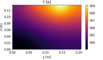
    # temperature
    plt.subplot(224)
    T_plot = plt.pcolormesh(
        y_plot, z_plot, T(y=y_plot, z=z_plot, t=t).T, shading="gouraud"
    )
    plt.axis([0, L_z, 0, L_z])
    plt.xlabel(r"$y$ [m]")
    plt.ylabel(r"$z$ [m]")
    plt.title(r"$T$ [K]")
    plt.set_cmap("inferno")
    plt.colorbar(T_plot)

    plt.subplots_adjust(
        top=0.92, bottom=0.15, left=0.10, right=0.9, hspace=0.5, wspace=0.5
    )
    plt.show()


# call plot with time in seconds
plot(1000)

you can evaluate the post-processed variables at any y, z, t.

[YouHyin]

First of all, thank you very much for letting me know

code

import pybamm
import numpy as np
import matplotlib.pyplot as plt

#pybamm.set_logging_level("INFO")

load model

options = {
"current collector": "potential pair",
"dimensionality": 2, # 2D current collectors
"thermal": "x-lumped", # thermal model (ignores through-cell variation)
}
model = pybamm.lithium_ion.SPM(options)

parameters can be updated here

param = model.default_parameter_values

set mesh points

var = pybamm.standard_spatial_vars
var_pts = {
var.x_n: 10, # negative electrode
var.x_s: 10, # separator
var.x_p: 10, # positive electrode
var.r_n: 10, # negative particle
var.r_p: 10, # positive particle
var.y: 10, # current collector y-direction
var.z: 10, # current collector z-direction
}

solver

solver = pybamm.CasadiSolver(atol=1e-6, rtol=1e-3, root_tol=1e-3, mode="fast")
experiment = pybamm.Experiment(
[
(

            "Charge at 2.5 C until 4.1 V",
            "Charge at 4.1 V until 50 mA",

        )
    ]
    ,
    termination="80% capacity",

)

simulation

simulation = pybamm.Simulation(
model, experiment=experiment, parameter_values=param, var_pts=var_pts, solver=solver
)

solve

#t_eval = np.linspace(0, 3600, 100) # time in seconds
simulation.solve()
solution = simulation.solution
solution(["Time [s]"]).entries[-1]

plotting ---------------------------------------------------------------------

post-process variables

phi_s_cn = solution["Negative current collector potential [V]"]
phi_s_cp = solution["Positive current collector potential [V]"]
I = solution["Current collector current density [A.m-2]"]
T = solution["X-averaged cell temperature [K]"]
print(solution"X-averaged cell temperature [K]")

mesh for plotting

L_y = param.evaluate(model.param.L_y)
L_z = param.evaluate(model.param.L_z)
y_plot = np.linspace(0, L_y, 21)
z_plot = np.linspace(0, L_z, 21)

Questions

1. I want to find the total charging time. So I write solution[“Time [s]”]. entries[-1] But simulation.solve() This code is getting an error. how can it be resolved??? Also, to find the charging time, can I write solution[“Time [s]”]. entries[-1]?
2. I want to know the temperature value of a specific time, so I enter the code solution["X-averaged cell temperature [K]"(t), but I get an error. What should I do if I want to know the temperature at a specific time as a value?

[rtimms]

1. is related to this issue - experiments don't work with 2D current collectors right now
2. you need to do solution["X-averaged cell temperature [K]"](y=y_plot, z=z_plot, t=t)