elegansAlignmentCountTable.Rmd

---
title: "Elegans: Read Alignment and Count Table with QausR and Rhisat2"
author: "Lieven Clement"
date: "statOmics, Ghent University (https://statomics.github.io)"
output:
    html_document:
      code_download: true
      theme: flatly
      toc: true
      toc_float: true
      highlight: tango
      number_sections: true
linkcolor: blue
urlcolor: blue
citecolor: blue
---

```{r, echo=FALSE}
suppressPackageStartupMessages({
  library(tidyverse)
  library(R.utils)
})
```
# Background 

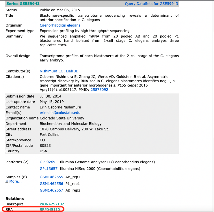
After fertilization but prior to the onset of zygotic transcription, the C. elegans zygote cleaves asymmetrically to create the anterior AB and posterior P1 blastomeres, each of which goes on to generate distinct cell lineages. To understand how patterns of RNA inheritance and abundance arise after this first asymmetric cell division, we pooled hand-dissected AB and P1 blastomeres and performed RNA-seq (Study [GSE59943](https://www.ncbi.nlm.nih.gov/geo/query/acc.cgi?acc=GSE59943)).


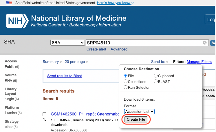
The information which connects the sample information from GEO with the SRA run id is downloaded from [SRA](https://www.ncbi.nlm.nih.gov/sra?term=SRP045110) using the Send to: File button.

![](https://raw.githubusercontent.com/statOmics/SGA/master/images_sequencing/elegans_GSE59943.png)

![](https://raw.githubusercontent.com/statOmics/SGA/master/images_sequencing/elegans_sraAccessions.png)

# Preprocessing 

## Download Data 

We used the info in the downloaded SraAccList.txt file to download the SRA files. 
We used the system function to invoke aan OS command. xargs can converts each line of a file into an argument. 

The fasterq-dump function will then download and convert each corresponding sra file from the SRA archive to a fastq file. 

The fasterq-dump is a tool from the [sra-tools](https://github.com/ncbi/sra-tools) suite that can be used to download sra files and to convert them into the fastq format. 

```
system("xargs fasterq-dump -p < SraAccList.txt")
```

For illustration purposes we will download subsampled fastq files from the course github site. 


```{r}
timeout <- options()$timeout
options(timeout = 300) #prevent timeout

url <- "https://github.com/statOmics/SGA/archive/refs/heads/elegansFastq.zip"
destFile <- "elegansFastq.zip"

download.file(url, destFile)

unzip(destFile, exdir = "./", overwrite = TRUE)

if (file.exists(destFile)) {
  #Delete file if it exists
  file.remove(destFile)
}

options(timeout = timeout) #prevent timeout
```

## Assess Read Quality 

Assess the fastq files with [fastQC](https://www.bioinformatics.babraham.ac.uk/projects/fastqc/). 

## Align data

### Input file for hisat aligner

We will make the input file for the hisat aligner that will be called through the QUASAR package. 

```{r}
fastqFiles <- list.files(path = "SGA-elegansFastq",full.names = TRUE, pattern = "fastq")

samples <- fastqFiles |>
    substr(start=18,stop=27) 
fileInfo <- tibble(FileName=fastqFiles,SampleName=samples)
fileInfo
```

We write the fileInfo to disk 

```{r}
write_tsv(fileInfo,file="fastQfiles.txt")
```

### Download C. elegans genome and gff3 file 

```{r refGenome, echo=FALSE, fig.cap="slide courtesy Charlotte Soneson", out.width='100%'}
knitr::include_graphics("https://raw.githubusercontent.com/statOmics/SGA/master/images_sequencing/humanReferenceGenome_fig.png")
```


```{r refTranscriptome, echo=FALSE, fig.cap="slide courtesy Charlotte Soneson", out.width='100%'}
knitr::include_graphics("https://raw.githubusercontent.com/statOmics/SGA/master/images_sequencing/humanReferenceTranscriptome_fig.png")
```

```{r}
urlGenome <- "https://ftp.ensembl.org/pub/release-108/fasta/caenorhabditis_elegans/dna/Caenorhabditis_elegans.WBcel235.dna.toplevel.fa.gz"
genomeDestFile <- "Caenorhabditis_elegans.WBcel235.dna.toplevel.fa.gz"
urlGff <- "https://ftp.ensembl.org/pub/release-108/gff3/caenorhabditis_elegans/Caenorhabditis_elegans.WBcel235.108.gff3.gz"
gffDestFile <- "Caenorhabditis_elegans.WBcel235.108.gff3.gz"

download.file(url = urlGenome ,
              destfile = genomeDestFile)
download.file(url = urlGff,
              destfile = gffDestFile)
gunzip(genomeDestFile, overwrite = TRUE, remove=TRUE)
gunzip(gffDestFile, overwrite = TRUE, remove=TRUE)
list.files()
```

### Align reads using QuasR and RHisat package

- We are aligning RNA-seq reads and have to use a gap aware alignment modus. We therefore use the argument `splicedAlignment = TRUE`

- The project is a single-end sequencing project! So we use the argument `paired = "no"`.

```{r}
suppressPackageStartupMessages({
    library(QuasR)
    library(Rhisat2)
})
sampleFile <- "fastQfiles.txt"
genomeFile <- "Caenorhabditis_elegans.WBcel235.dna.toplevel.fa"    
projElegans <- qAlign(
    sampleFile = sampleFile, 
    genome = genomeFile,
    splicedAlignment = TRUE, 
    aligner = "Rhisat2",
    paired="no")
```

## Make count table

### Convert gff file into database

The gff3 file contains information on the position of features, e.g. exons and genes, along the chromosome. 

```{r}
suppressPackageStartupMessages({
library(GenomicFeatures)
library(Rsamtools)
})
annotFile <- "Caenorhabditis_elegans.WBcel235.108.gff3"

#chrLen <- scanFaIndex(genomeFile)

#chrominfo <- data.frame(chrom = as.character(seqnames(chrLen)),
#                        length = width(chrLen),
#                        is_circular = rep(FALSE, length(chrLen)))

txdb <- makeTxDbFromGFF(file = annotFile,
                        dataSource = "Ensembl",
                        organism = "Caenorhabditis elegans")
```

### Make Gene Count table 

With the qCount function we can count the overlap between the aligned reads and the genomic features of interest. 

```{r}
geneCounts <- qCount(projElegans, txdb, reportLevel = "gene")
head(geneCounts)
```

Save count table for future use. 

```{r}
write.csv(as.data.frame(geneCounts),file = "elegansCountTable.csv")
```


# Session Info

With respect to reproducibility, it is highly recommended to include a session info in your script so that readers of your output can see your particular setup of R. 

```{r}
sessionInfo()
```