The main difference between the two types is that supervised learning is done using a ground truth, or in other words, we have prior knowledge of what the output values for our samples should be. Therefore, the goal of supervised learning is to learn a function that, given a sample of data and desired outputs, best approximates the relationship between input and output observable in the data.
Unsupervised learning, on the other hand, does not have labeled outputs, so its goal is to infer the natural structure present within a set of data points. We wish to learn the inherent structure of our data without using explicitly-provided labels.
Bias is the difference between the average prediction of our model and the correct value which we are trying to predict. Model with high bias pays very little attention to the training data and oversimplifies the model. It always leads to high error on training and test data, meaning that the model underfits on the training data.
Variance is the variability of model prediction for given data points or a value which tells us spread of our data. Model with high variance pays a lot of attention to training data and does not generalize on the data which it hasn’t seen before. As a result, such models perform very well on training data but has high error rates on test data, meaning thet the model overfits on the training data.
What we desire is low bias, low variance. But there is a bias-variance tradeoff.
The simpler the model, the higher the bias, and the more complex the model, the higher the variance. If our model is too simple and has very few parameters then it may have high bias and low variance. On the other hand if our model has large number of parameters then it’s going to have high variance and low bias. So we need to find the right/good balance without overfitting and underfitting the data. This tradeoff in complexity is why there is a tradeoff between bias and variance.
Underfitting happens when a model unable to capture the underlying pattern of the data. These models usually have high bias. It happens when we have very less amount of data to build an accurate model or when we try to build a simpler model to capture more complex patterns in data, for eg a linear model with nonlinear data, say a linear regression model for y = x^2 + error
Overfitting happens when we achieve a good fit of your model on the training data, while it does not generalize well on new, unseen data. The model tends to capture the noise along with the underlying pattern in data. It happens when we train our model a lot over noisy dataset, or build models complex enough that tend to learn the noise in the data as well or at times even just memorize the training data. These models have low bias and high variance.
By noise we mean the data points that don’t really represent the true properties of your data, but random chance.
- The best option is to get more training data. Unfortunately, in real-world situations, you often do not have this possibility due to time, budget, or technical constraints.
- To lower the capacity of the model to memorize the training data. As such, the model will need to focus on the relevant patterns in the training data, which results in better generalization. This can be done by removing layers or reducing the number of elements in the hidden layers
- Apply regularization, which adds a cost to the loss function penalizing for large weights. Popular ones are L1 and L2
- Use Dropout layers, which will randomly remove certain features by setting them to zero
- Batch normalization
L1 regularization will add a cost with regards to the absolute value of the parameters. It will result in some of the weights to be equal to zero. Also used for feature selection
L2 regularization will add a cost with regards to the squared value of the parameters. This results in smaller weights.
Medium: https://towardsdatascience.com/ridge-and-lasso-regression-a-complete-guide-with-python-scikit-learn-e20e34bcbf0b
Dropout is a technique meant to prevent overfitting the training data by dropping out units in a neural network. In practice, neurons are either dropped with probability p or kept with probability 1-p
- Faster model
- Easier to understand / interpretable model
- Better performing model
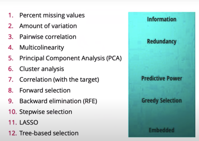
- Percent missing values: Features that have many missing values are hard to learn from
- Amount of variation: If a feature is mostly all the same value, then the model is not going to learn anything from it
- Pairwise correlation: If two features are highly correlated, we can drop one since its redundant. So if we drop one, we won’t actually be losing that much information in terms of what the model can learn from
- Multicolinarity
- PCA
- Cluster analysis
- Correlation (with target): If a variable has a very low correlation with the target, then we can probably drop it. Might drop a useful feature though
- Forward selection: Iteratively add the best feature until some threshold
- Backward elimination: Iteratively drop the worst feature until some threshold
- Stepwise elimination: Combination of forward and backward
- LASSO: Least absolute shrinkage and selection operator
- Tree based selection: Forests of trees to evaluate the importance of features
Youtube: https://youtu.be/YaKMeAlHgqQ
An ROC curve (receiver operating characteristic curve) is a graph showing the performance of a classification model at all classification thresholds. This curve plots two parameters, True Positive Rate (recall) and False Positive Rate at different classification thresholds. Lowering the classification threshold classifies more items as positive, thus increasing both False Positives and True Positives.
To compute the points in an ROC curve, we could evaluate a model many times with different classification thresholds, but this would be inefficient. Fortunately, there's an efficient, sorting-based algorithm that can provide this information for us, called AUC.
That is, AUC measures the entire two-dimensional area underneath the entire ROC curve (think integral calculus) from (0,0) to (1,1).
Interpretation:
AUC provides an aggregate measure of performance across all possible classification thresholds. One way of interpreting AUC is as the probability that the model ranks a random positive example more highly than a random negative example.
AUC is desirable for the following two reasons:
AUC is scale-invariant. It measures how well predictions are ranked, rather than their absolute values. AUC is classification-threshold-invariant. It measures the quality of the model's predictions irrespective of what classification threshold is chosen.
However, both these reasons come with caveats, which may limit the usefulness of AUC in certain use cases:
Scale invariance is not always desirable. For example, sometimes we really do need well calibrated probability outputs, and AUC won’t tell us about that.
Classification-threshold invariance is not always desirable. In cases where there are wide disparities in the cost of false negatives vs. false positives, it may be critical to minimize one type of classification error. For example, when doing email spam detection, you likely want to prioritize minimizing false positives (even if that results in a significant increase of false negatives). AUC isn't a useful metric for this type of optimization.
Medium: https://towardsdatascience.com/understanding-auc-roc-curve-68b2303cc9c5#:~:text=AUC%20%2D%20ROC%20curve%20is%20a,problem%20at%20various%20thresholds%20settings.&text=By%20analogy%2C%20Higher%20the%20AUC,is%20on%20the%20x%2Daxis.
The “No Free Lunch” theorem states that there is no one model that works best for every problem. The assumptions of a great model for one problem may not hold for another problem, so it is common practice to try multiple models and find one that works best for the particular problem and data in hand.
The core idea is that we cannot know exactly how well an algorithm will work in practice (the true "risk") because we don't know the true distribution of data that the algorithm will work on, but we can instead measure its performance on a known set of training data (the "empirical" risk). Empirical risk minimization is a principle in statistical learning theory which defines a family of learning algorithms and is used to give theoretical bounds on their performance.
- Class weighting
- Sampling techniques
- Generate synthetic samples
- Stratified test split
- F1 score
- Dice loss : Dice loss is based on the Sørensen–Dice coefficient (Sorensen, 1948) or Tversky index (Tversky, 1977), which attaches similar importance to false positives and false negatives, and is more immune to the data-imbalance issue
- K fold cross validation
Selection bias occurs if a data set's examples are chosen in a way that is not reflective of their real-world distribution. Selection bias can take many different forms: coverage bias, sampling bias, participation bias (non-response bias).
Random forest (RF) is an ensemble method that uses multiple models of several DTs to obtain a better prediction performance. It creates many classification trees and a bootstrap sample technique is used to train each tree from the set of training data.
“It is a tree-based technique that uses a high number of decision trees built out of randomly selected sets of features. Contrary to the simple decision tree, it is highly uninterpretable but its generally good performance makes it a popular algorithm.”
Randomness is introduced in the selection of features for each tree. Instead of searching for the most important feature while splitting a node, the algorithm selects a random set of features for splitting a node for each tree generated. This allows the model to be more diverse, flexible, factor chaos as well as experience a less deterministic structure that allows to outperform out-of-sample and minimize the risk of overfitting.
A logistic regression model is searching for a single linear decision boundary in your feature space, whereas a decision tree is essentially partitioning your feature space into half-spaces using axis-aligned linear decision boundaries. The net effect is that you have a non-linear decision boundary, possibly more than one.
This is nice when your data points aren't easily separated by a single hyperplane, but on the other hand, decisions trees are so flexible that they can be prone to overfitting. To combat this, you can try pruning. Logistic regression tends to be less susceptible (but not immune!) to overfitting.
Lastly, another thing to consider is that decision trees can automatically take into account interactions between variables, e.g. 𝑥𝑦 if you have two independent features 𝑥 and 𝑦. With logistic regression, you'll have to manually add those interaction terms yourself.
Both are supervised machine learning algorithms.
Logistic regression is an algorithm that is used in solving classification problems. It uses logistic (sigmoid) function to find the relationship between variables. The sigmoid function is an S-shaped curve that can take any real-valued number and map it to a value between 0 and 1, but never exactly at those limits.
SVM is a model used for both classification and regression problems though it is mostly used to solve classification problems. The algorithm creates a hyperplane or line(decision boundary) which separates data into classes. It finds the “best” hyperplane that could maximize the margin between the classes, which means that the distance between the hyperplane and the nearest data points on each side is the largest. It uses the kernel trick to find the best line separator (decision boundary that has same distance from the boundary point of both classes, these boundary points are called the support vectors). It is a more powerful way of learning complex non-linear functions.
- SVM tries to finds the “best” margin (distance between the line and the support vectors) that separates the classes and this reduces the risk of error on the data, while logistic regression does not, instead it can have different decision boundaries with different weights that are near the optimal point.
- SVM works well with unstructured and semi-structured data like text and images while logistic regression works with already identified independent variables.
- SVM is based on geometrical properties of the data while logistic regression is based on statistical approaches.
n = number of features, m = number of training examples
- If n is large (1–10,000) and m is small (10–1000) : use logistic regression or SVM with a linear kernel.
- If n is small (1–10 00) and m is intermediate (10–10,000) : use SVM with (Gaussian, polynomial etc) kernel
- If n is small (1–10 00), m is large (50,000–1,000,000+): first, manually add more features and then use logistic regression or SVM with a linear kernel
Also if we strong reasons to believe that the data wont be linearly separable, its a good idea to use an SVM with a nonlinear kernel
Kernel trick is widely used to bridge linearity and non-linearity. It offers a more efficient and less expensive way to transform data into higher dimensions. The goal is to map the original non-linear observations into a higher-dimensional space in which they become separable. However, when there are more and more dimensions, computations within that space become more and more expensive. This is when the kernel trick comes in. It allows us to operate in the original feature space without computing the coordinates of the data in a higher-dimensional space.
The kernel trick sounds like a “perfect” plan. However, one critical thing to keep in mind is that when we map data to a higher dimension, there are chances that we may overfit the model. Thus choosing the right kernel function (including the right parameters) and regularization are of great importance.
We say that we use the "kernel trick" to compute the cost function using the kernel because we actually don't need to know the explicit feature mapping ϕ, which is often very complicated. Instead, only the values K(x,z) are needed. K(x,z) = ϕ(x)^Tϕ(z)
A parametric algorithm has a fixed number of parameters. A parametric algorithm is computationally faster, but makes stronger assumptions about the data; the algorithm may work well if the assumptions turn out to be correct, but it may perform badly if the assumptions are wrong. A common example of a parametric algorithm is linear regression.
In contrast, a non-parametric algorithm uses a flexible number of parameters, and the number of parameters often grows as it learns from more data. A non-parametric algorithm is computationally slower, but makes fewer assumptions about the data. A common example of a non-parametric algorithm is K-nearest neighbour.
To summarize, the trade-offs between parametric and non-parametric algorithms are in computational cost and accuracy.
“Birds with similar features flock together”
Advantages:
- k-NN is a simple and intuitive supervised algorithm
- Non-parametric algorithm
- Fast prototyping and data analyses
Disadvantages:
- Slow
- Imbalance data : kNN doesn’t perform well on imbalanced data. If we consider two classes, A and B, and the majority of the training data is labeled as A, then the model will ultimately give a lot of preference to A. This might result in getting the less common class B wrongly classified.
- Outlier sensitivity: KNN algorithm is very sensitive to outliers as it simply chose the neighbors based on distance criteria.
- K value
Steps:
- Decide on your similarity or distance metric.
- Split the original labeled dataset into training and test data.
- Pick an evaluation metric.
- Decide upon the value of k. Here k refers to the number of closest neighbors we will consider while doing the majority voting of target labels. The higher the parameter k, the higher the bias, and the lower the parameter k, the higher the variance.
- Run k-NN a few times, changing k and checking the evaluation measure.
- In each iteration, k neighbors vote, majority vote wins and becomes the ultimate prediction
- Optimize k by picking the one with the best evaluation measure.
- Once you’ve chosen k, use the same training set and now create a new test set, and want to predict.
Python code (from scratch): https://medium.com/roottech/knn-understanding-k-nearest-neighbor-algorithm-in-python-71488b8802f0
Fit and Inefficiency stackexchange: https://stats.stackexchange.com/questions/349842/why-do-we-need-to-fit-a-k-nearest-neighbors-classifier#:~:text=Fitting%20a%20classifier%20means%20taking,a%20space%20of%20possible%20classifiers.&text=But%2C%20in%20the%20case%20of,requires%20storing%20the%20training%20set.
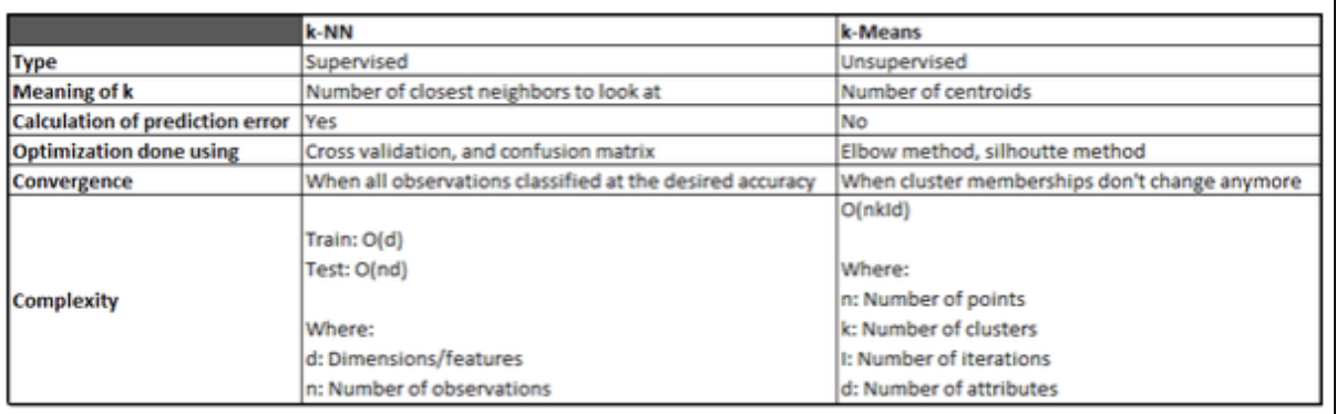
k-Means is an unsupervised algorithm used for clustering. We don’t have any labeled data upfront to train the model. Hence the algorithm just relies on the dynamics of the input features to make inferences on unseen data.
Steps:
- Initially, randomly pick k centroids/cluster centers. Try to make them near the data but different from one another.
- Find the Euclidean distance of each point in the data set with the identified K points — cluster centroids.
- Then assign each data point to the closest centroid using the distance found.
- Calculate new centroids by taking the average of the points in each cluster group.
- Repeat the preceding 3 steps for a fixed number of iterations or until the assignments don’t change, or change very little.
Finding K in K means: To do this we have many algorithms like cross validation, bootstrap, AUC, BIC and many more. But we will discuss one of the most simple and easy to comprehend algorithm called “elbow point”. The basic idea behind this algorithm is that it plots the various values of cost with changing k. As the value of K increases, there will be fewer elements in the cluster. So average distortion will decrease. The lesser number of elements means closer to the centroid. So, the point where this distortion declines the most is the elbow point and that will be our optimal K.
Python code (from scratch) and details: https://medium.com/@rishit.dagli/build-k-means-from-scratch-in-python-e46bf68aa875
K-means is a clustering algorithm that tries to partition a set of points into K sets (clusters) such that the points in each cluster tend to be near each other. It is unsupervised because the points have no external classification.
K-nearest neighbors is a classification (or regression) algorithm that in order to determine the classification of a point, combines the classification of the K nearest points. It is supervised because you are trying to classify a point based on the known classification of other points.
Quora: https://www.quora.com/How-is-the-k-nearest-neighbor-algorithm-different-from-k-means-clustering
Smoothing is a technique applied to time series to remove the fine-grained variation between time steps, to reduce the random variation in the observations, a statistical approach of eliminating outliers from datasets to make the patterns more noticeable. The hope is to remove noise and better expose the signal of the underlying causal processes.
Moving averages are a simple and common type of smoothing used in time series analysis and time series forecasting. Calculating a moving average involves creating a new series where the values are comprised of the average of raw observations in the original time series. A moving average requires that you specify a window size called the window width. This defines the number of raw observations used to calculate the moving average value. The “moving” part in the moving average refers to the fact that the window defined by the window width is slid along the time series to calculate the average values in the new series.
Calculating a moving average of a time series makes some assumptions about your data. It is assumed that both trend and seasonal components have been removed from your time series. This means that your time series is stationary, or does not show obvious trends (long-term increasing or decreasing movement) or seasonality (consistent periodic structure). There are many methods to remove trends and seasonality from a time series dataset when forecasting. Two good methods for each are to use the differencing method and to model the behavior and explicitly subtract it from the series.
Centered Moving Average: The value at time (t) is calculated as the average of raw observations at, before, and after time (t). This method requires knowledge of future values, hence cannot use when forecasting.
Trailing Moving Average: The value at time (t) is calculated as the average of the raw observations at and before the time (t). Trailing moving average only uses historical observations and is used on time series forecasting.
Note: The rolling() function on the Series Pandas object
Moving Average: https://machinelearningmastery.com/moving-average-smoothing-for-time-series-forecasting-python/
Pandas rolling() function: http://pandas.pydata.org/pandas-docs/stable/generated/pandas.Series.rolling.html
Exponential Moving Average (EMA): https://towardsdatascience.com/trading-toolbox-02-wma-ema-62c22205e2a9
Different Smoothing techniques: https://corporatefinanceinstitute.com/resources/knowledge/other/data-smoothing/
Disadvantages of data smoothing:
- Data smoothing does not necessarily offer an interpretation of the themes or patterns it helps to recognize. It can also contribute to certain data points being overlooked by focusing on others.
- Sometimes, data smoothing may eliminate the usable data points. It may lead to incorrect forecasts if the data set is seasonal and not completely be reflective of the reality produced by the data points. Moreover, data smoothing can be prone to considerable disruption from the outliers in the data.
Gradient descent is an iterative optimization algorithm for finding a local minimum of a differentiable function. The idea is to take repeated steps in the opposite direction of the gradient of the function at the current point, because this is the direction of steepest descent.
Backpropagation stands for “backward propagation of errors”. It is an algorithm for training neural networks using gradient descent. The method calculates the gradient of the error function with respect to the neural network's weights. Simply put, backpropagation finds the derivatives of the network by moving layer by layer from the final layer to the initial one. By the chain rule, the derivatives of each layer are multiplied down the network (from the final layer to the initial) to compute the derivatives of the initial layers.
Regularization discourages learning a more complex model, so as to avoid the risk of overfitting and reduce variance of the model. This can be done by adding an additional term in the loss function penalizing the model for complexity. Other recent approaches like dropout have shown regularization properties, and even batch normalization arguably.
Let's take a second to imagine a scenario in which you have a very simple neural network with two inputs. The first input value, x1, varies from 0 to 1 while the second input value, x2, varies from 0 to 0.01. Since your network is tasked with learning how to combine these inputs through a series of linear combinations and nonlinear activations, the parameters associated with each input will also exist on different scales.
Unfortunately, this can lead toward an awkward loss function topology which places more emphasis on certain parameter gradients.
By normalizing all of our inputs to a standard scale, we're allowing the network to more quickly learn the optimal parameters for each input node.
Additionally, it's useful to ensure that our inputs are roughly in the range of -1 to 1 to avoid weird mathematical artifacts associated with floating-point number precision. In short, computers lose accuracy when performing math operations on really large or really small numbers. Moreover, if your inputs and target outputs are on a completely different scale than the typical -1 to 1 range, the default parameters for your neural network (ie. learning rates) will likely be ill-suited for your data.
Motivation: We normalize the input layer by adjusting and scaling the activations. For example, when we have features from 0 to 10 and some from 1 to 10k, we should normalize them to speed up learning and other reasons I can detail if you’d like. But basically, If the input layer is benefiting from it, why not do the same thing also for the values in the hidden layers, that are changing all the time, and get more improvement in the training speed.
Why
- Batch normalization reduces the amount by what the hidden unit values shift around (covariance shift). It increases the stability of an NN in a way.
- Also, batch normalization allows each layer of a network to learn by itself a little bit more independently of other layers.
- Since batch normalization makes sure that there’s no activation that’s gone really high or really low, we can use higher learning rates. And by that, things that previously couldn’t get to train, it will start to train.
- From my personal experience, Parkinson’s project exploding gradients nan → batch normalization did the trick.
- It reduces overfitting because it has slight regularization effects as it adds some noise to each hidden layer’s activations. But recent papers arguably suggest why batch norm shouldn’t be used explicitly for regularization
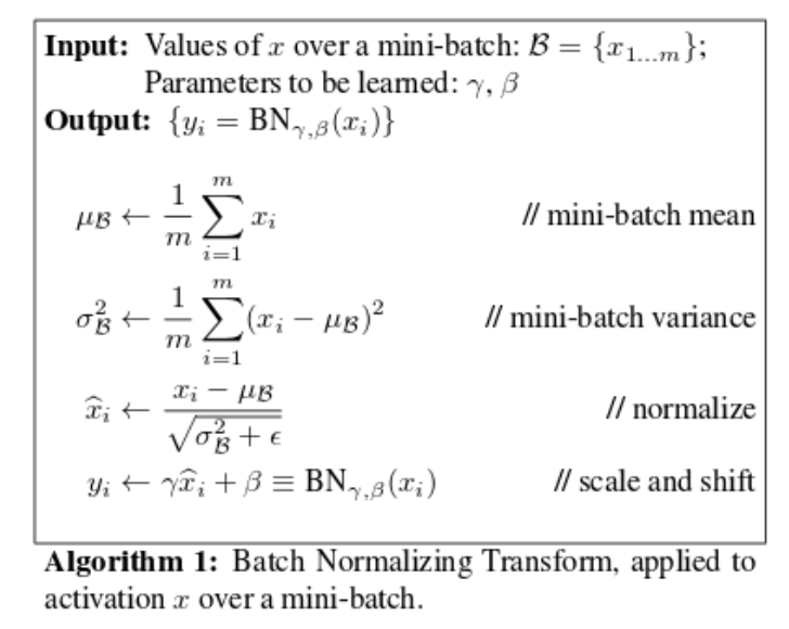
How To increase the stability of a neural network, batch normalization normalizes the output of a previous activation layer by subtracting the batch mean and dividing by the batch standard deviation.
However, after this shift/scale of activation outputs by some randomly initialized parameters, the weights in the next layer are no longer optimal. SGD ( Stochastic gradient descent) undoes this normalization if it’s a way for it to minimize the loss function.
Consequently, batch normalization adds two trainable parameters to each layer, so the normalized output is multiplied by a “standard deviation” parameter (gamma) and add a “mean” parameter (beta). In other words, batch normalization lets SGD do the denormalization by changing only these two weights for each activation, instead of losing the stability of the network by changing all the weights.
When training a deep neural network with gradient based learning and backpropagation, we find the partial derivatives by traversing the network from the the final layer (y_hat) to the initial layer. Using the chain rule, layers that are deeper into the network go through continuous matrix multiplications in order to compute their derivatives.
In a network of n hidden layers, n derivatives will be multiplied together. If the derivatives are small then the gradient will decrease exponentially as we propagate through the model until it eventually become too small to train the model effectively, or vanishes, and this is the vanishing gradient problem.
The accumulation of small gradients results in a model that is incapable of learning meaningful insights since the weights and biases of the initial layers, which tends to learn the core features from the input data (X), will not be updated effectively. In the worst case scenario the gradient will be 0 which in turn will stop the network will stop further training.
How to identify
- The model will improve very slowly during the training phase and it is also possible that training stops very early, meaning that any further training does not improve the model.
- The weights closer to the output layer of the model would witness more of a change whereas the layers that occur closer to the input layer would not change much (if at all).
- Model weights shrink exponentially and become very small when training the model.
- The model weights become 0 in the training phase.
Solutions:
- Reducing the number of layers but giving up complexity might hurt the model’s performance to find complex mappings.
- The simplest solution is to use other activation functions, such as ReLU, which doesn’t cause a small derivative.
- Residual networks or skip connections are another solution, as they provide residual or skip connections straight to earlier layers. If we consider a residual block, the residual connection directly adds the value at the beginning of the block, x, to the end of the block (F(x)+x). This residual connection doesn’t go through activation functions that “squashes” the derivatives, resulting in a higher overall derivative of the block.
- Batch normalization layers can also help resolve the issue. As stated before, the problem arises when a large input space is mapped to a small one, causing the derivatives to disappear. Eg, for sigmoid activation, when |x| is big. Batch normalization reduces this problem by simply normalizing the input so |x| doesn’t reach the outer edges of the sigmoid function, and the derivative isn’t too small.
- A more careful initialization choice of the random initialization for the network tends to be a partial solution, since it does not solve the problem completely.
When training a deep neural network with gradient based learning and backpropagation, we find the partial derivatives by traversing the network from the the final layer (y_hat) to the initial layer. Using the chain rule, layers that are deeper into the network go through continuous matrix multiplications in order to compute their derivatives.
In a network of n hidden layers, n derivatives will be multiplied together. If the derivatives are large then the gradient will increase exponentially as we propagate down the model until they eventually explode, and this is what we call the problem of exploding gradient.
In the case of exploding gradients, the accumulation of large derivatives results in the model being very unstable and incapable of effective learning, The large changes in the models weights creates a very unstable network, which at extreme values the weights become so large that is causes overflow resulting in NaN weight values of which can no longer be updated.
How to identify:
- The model is not learning much on the training data therefore resulting in a poor loss
- The model will have large changes in loss on each update due to the models instability
- The models loss will be NaN during training
Confirmation:
- Model weights grow exponentially and become very large when training the model
- The model weights become
nanin the training phase - The derivatives are constantly increasing
Solutions:
- Reducing the number of layers but giving up complexity might hurt the model’s performance to find complex mappings
- Gradient clipping: Checking for and limiting the size of the gradients whilst our model trains
- A more careful initialization choice of the random initialization for your network tends to be a partial solution, since it might not solve the problem completely
- Batch normalization layers can also help resolve the issue