An algorithm is a set of instructions to solve a problem. It is a sequence of steps that are followed in order to solve a problem. Algorithms are used in many areas of computer science, such as data structures, artificial intelligence, and computer graphics.
Algorithms have the following properties:
- Input: An algorithm takes zero or more inputs.
- Output: An algorithm produces one or more outputs.
- Definiteness: Each step of an algorithm must be clear and unambiguous.
- Finiteness: An algorithm must terminate after a finite number of steps.
- Effectiveness: An algorithm must be effective in solving the problem for which it is designed.
There are many types of algorithms, such as:
- Brute Force: An algorithm that tries all possible solutions to a problem.
- Greedy: An algorithm that makes the best choice at each step.
- Divide and Conquer: An algorithm that breaks a problem into smaller subproblems.
- Dynamic Programming: An algorithm that solves a problem by solving smaller subproblems.
- Backtracking: An algorithm that tries all possible solutions and backtracks when it reaches a dead end.
- Randomized: An algorithm that uses random numbers to make decisions.
- Approximation: An algorithm that finds an approximate solution to a problem.
- Heuristic: An algorithm that uses a rule of thumb to find a good solution.
The complexity of an algorithm is a measure of the amount of resources it consumes, such as time and space. There are two types of complexity:
-
Time Complexity: The amount of time an algorithm takes to run as a function of the size of the input.
-
Space Complexity: The amount of memory an algorithm uses as a function of the size of the input.
The complexity of an algorithm is usually expressed using big O notation, which describes the upper bound on the growth rate of the algorithm.
Learn more about Big O Notation, and see the Big O Cheat Sheet for common algorithms and their complexities.
Each of these approaches could be called algorithms. The speed of each of these algorithms can be pictured as follows in what is called big-O notation:
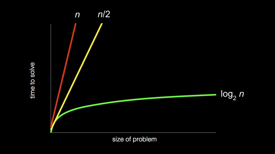
Notice that the first algorithm, highlighted in red, has a big-O of n because if there are 100 names in the phone book, it could take up to 100 tries to find the correct name. The second algorithm, where two pages were searched at a time, has a big-O of ‘n/2’ because we searched twice as fast through the pages. The final algorithm has a big-O of log2n as doubling the problem would only result in one more step to solve the problem.
-
O(1): Constant time complexity. The algorithm takes the same amount of time to run, regardless of the size of the input.
-
O(log n): Logarithmic time complexity. The algorithm's running time grows logarithmically as the size of the input grows.
-
O(n): Linear time complexity. The algorithm's running time grows linearly as the size of the input grows.
-
O(n log n): Linearithmic time complexity. The algorithm's running time grows linearithmically as the size of the input grows.
-
O(n^2): Quadratic time complexity. The algorithm's running time grows quadratically as the size of the input grows.
-
O(2^n): Exponential time complexity. The algorithm's running time grows exponentially as the size of the input grows.
-
O(n!): Factorial time complexity. The algorithm's running time grows factorially as the size of the input grows.
The analysis of algorithms is the study of the performance of algorithms. It involves measuring the time and space complexity of algorithms and comparing them to other algorithms. The goal of algorithm analysis is to determine the best algorithm for a given problem.