- Powerful classification algorithm
- Finds best possible boundary among the model and classes
- Maintains the largest distance from the datapoint
In this project, we are going to classify the species of Iris flower. To view the project Click Here
Seaborn has some datasets, from that we are loading the Iris dataset.
iris = sns.load_dataset('iris')
import pandas as pd
import numpy as np
import seaborn as sns
import matplotlib.pyplot as plt
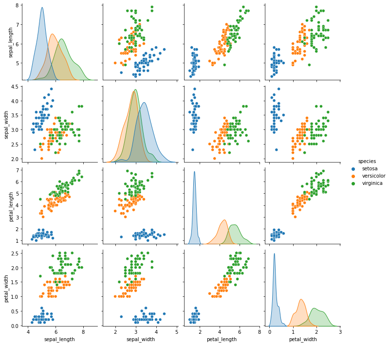
### EDA (Exploratory Data Analysis)
Pairplot is used, to get a glance at the relations of each feature. We can easily see which features are affecting one another.
Dividing our dataset for training and testing.
X is input and Y is output.
from sklearn.model_selection import train_test_split
x = iris.drop('species',axis = 1)
y = iris['species']
xtrain , xtest , ytrain ,ytest = train_test_split(x , y , test_size = 0.3)
Creating an instance of the model and fitting it.
from sklearn.svm import SVC
svm = SVC()
svm.fit(xtrain ,ytrain)
Seeing the performance of the model using confusion matrix and classification report.
pred = svm.predict(xtest)
from sklearn.metrics import classification_report,confusion_matrix
print(confusion_matrix(ytest,pred))
print(classification_report(ytest,pred))
Let's import grid search and create a dictionary with all the parameters like C, kernel, gamma.
from sklearn.model_selection import GridSearchCV
param_grid = {'C':[0.01,0.1,1,10,100,1000], 'gamma':[1000,100,10,1,0.1,0.01], 'kernel':['rbf']}
Fitting Grid Search in the training data. The parameters are the instance of our model, the dictionary with parameters, refit, and verbose.
grid = GridSearchCV(SVC(),param_grid,refit = True , verbose = 3)
grid.fit(xtrain,ytrain)
Finding out which parameters worked out well with grid.best_params_
We are making a prediction and getting an insight from the confusion matrix and classification report after tuning the parameters.
Thank you!