Python tight binding

sids implements an easy data object for creating tight-binding models.

The easiest way to describe the tight-binding model is showcase its usage.

Graphene bandstructure

The graphene structure is one of the easiest structures to describe and provide tight-binding parameters for.

Nearest neighbour

First we create the geometry with nearest neighbour interactions

import sids
# Lattice constant
alat = 1.42
length = ( 1.5 ** 2 + 3. / 4. ) ** .5 * alat
C = sids.Atom(6,R=alat+0.1) # add small number for numerics
sc = sids.SuperCell([length,length,10,90,90,60],nsc=[3,3,1])
# Rotate supercell as the initial one is x = cartesian
sc = sc.rotate(-30,v=[0,0,1])
gr = sids.Geometry([[0,0,0],[1,0,0]], atoms=C, sc=sc)

which now results in a graphene unit cell with appropriate periodicity for nearest neighbour interactions.

We now proceed to create the tight-binding object

tb = sids.TightBinding(gr)

now we have a tight-binding object, but no hopping integrals or on-site energies have been set.

# Denote interactions ranges
#     on-site , nearest neighbour
dR = (0.1     , alat + 0.1)
for ia in gr:
    # Get interacting atoms
    idx = gr.close(ia, dR=dR)
    tb[ia,idx[0]] = ( 0. , 1.)
    tb[ia,idx[1]] = (-2.7, 0.)

there are a few things going on here:

1. dR is an array of arbitrary length which can be understood as spherical radii for returning the atoms close to another atom or position.

   The array can be arbitrarily long and returns a list of equal length with each list entry contain all entries in the spherical shell defined by the previous radii and the current radii.

   In the above code idx returned from close is

   • idx[0] all atoms with distance <= .1 of atom ia
   • idx[1] all atoms 0.1 < distance <= alat + 0.1 of atom ia

2. tb[ia,idx[0]] = (0.,1.) sets the on-site energy to 0 and the overlap matrix to 1.

3. tb[ia,idx[1]] = (-2.7,0) sets the nearest neighbour hopping integral to -2.7 and the overlap matrix to 0, hence yielding an orthogonal tight-binding model.

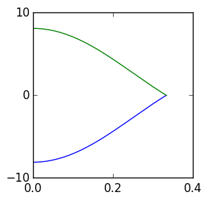
To finalise the bandstructure we calculate the bandstructure from \Gamma to K (so not full band-structure).

nk = 200
kpts = np.linspace(0, 1./3, nk)
eigs = np.empty([nk,2],np.float64)
for ik, k in enumerate(kpts):
    eigs[ik,:] = tb.eigh(k=[k,-k,0])

import matplotlib.pyplot as plt
plt.plot(kpts,eigs[:,0])
plt.plot(kpts,eigs[:,1])
plt.show()

Which results in this band-structure

Press this source link to get the complete source.