This is the final project for the Udacity Machine Learning Engineer with Microsoft Azure Nanodegree Program. In this project I will attempt to predict whether a tumor in a patient's breast is benign or malignant. I have used a dataset from Kaggle based on a medical study done.
I will use two methods to create a machine learning model. The first method to create a machine learning model will be AutoML and the second method will be Hyperdrive. After creating a model from each of these methods, I will then deploy the model with the highest accuracy as a web service using an Azure Container Instance (ACI). therafter I will submit a request to the deployed web service and obtain a prediction whether the tumor tissue is benign or malignant. Finally I will convert the chosen model to an onnx model and terminate all services and compute resources.
The first step after setting up a workspace for Azure Machine Learning Studio is to add a compute instance in order to execute code in my Jupyter notebooks.
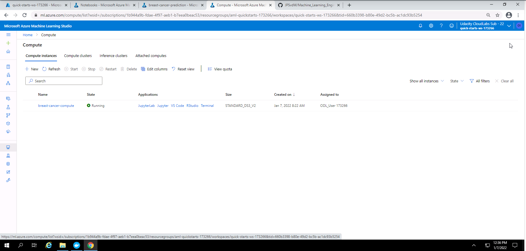
Screenshot 1: Compute instance.
Screenshot 1 shows that I have created a compute instance called "breast-cancer-compute". I used a STANDARD_DS3_V2 compute instance.
After the compute instance has been created, I uploaded my two Jupyter Notebooks called, "automl.ipynb" and "hyperparameter_tuning.ipynb".
In order to use the SKLearn estimator function in my "hyperparameter_tuning.ipynb" Notebook I had to create an entry script in python. My entry script name is "train.py". In this script I added:
- Dependencies that will be used.
- A method to download the dataset from Kaggle.com using Tabular Dataset Factory.
- Converted the data to a pandas dataframe.
- Cleaned the data.
- Split the dataset into a training and test dataset.
- Added the Logistic Regression model to be used along with a method to fetch the hyperparameters values provided in my "hyperparameter_tuning.ipynb" notebook.
The dataset is publicly available on the Kaggle website. The dataset was created from a study done on breast cancer. The attributes were created from a digitized image of a fine needle aspirate (FNA) of a breast mass. The end goal of this dataset is to predict whether the breast mass of a patient is malignant or benign. The dataset contains 30 attributes for each of the 569 patients and a single outcome or diagnosis.
A summary of the attributes is given below.
- radius (Distance from centre to the perimeter)
- texture (Standard deviation of gray-scale values)
- perimeter (Perimeter of tissue sample)
- area (Area of tissue sample)
- smoothness (Local variation in radius lenghts)
- compactness_mean (Perimeter^2/area - 1.0)
- concavity_mean (Severity of concave portions of the contour)
- concave points_mean (Number of concave portions of the contour)
- symmetry_mean (Symmetry of the tissue sample)
- fractal_dimension_mean ("Coastline approximation" - 1)
There are ten categories of features and for each of these categories, the mean, standard error and "worst" or largest (mean of the largest three values) were calculated to create a total of 30 features. The outcome or target field is the diagnosis which have a value of either malignant or benign.
The objective is tu use this dataset from Kaggle.com and create a trained machine learning model to predict whether the tissue sample taken from a tumor inside the breast of a patient is benign or malignant. A predicted outcome of 1 means malignant and a predicted outcome of 0 means benign.
This dataset was downloaded and uploaded to this repository from Kaggle.com and can be found at this link
- Tabular Dataset Factory is used to dowloaded and access the dataset from my repository in the data folder through a URL.
- The dataset was used in my "train.py" file and also in both my Jupyter Notebooks where I also show the first few lines of the dataset. I also show some statistics of my dataset in my Notebooks.
- In my "automl.ipynb" Notebook I had registered the dataset on Azure Machine Learning Studio.
In my "automl.ipynb" I executed a series of cells containing code that would create a machine learning model, save and register the best model from this experiment, and finaly deploy the model as the model with the best accuracy was obtained from the AutoML experiment. The following is an overview of cells that were executed:
- Import all dependencies that will be used in this notebook.
- Show my workspace, resource group, subscription details and choose a name for my experiment.
- Create an AML Compute cluster.

Screenshot 2: AML compute cluster created.
Screenshot 2 provides confirmation that the AML compute cluster was created successfully. This screen was accessed in the compute section of Azure Machine Learning Studio under the Compute clusters tab.
- Access the dataset from my Github repository and display the first few lines of the dataset and also some statistic on my dataset.
- Cleaning and registering of my dataset.
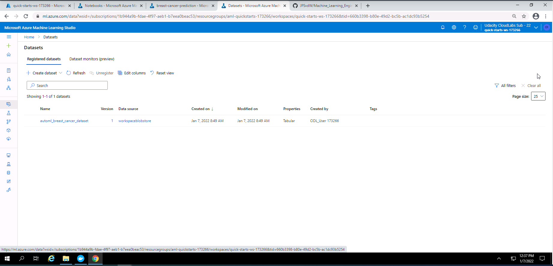
Screenshot 3: Registered dataset.
Screenshot 3 provides confirmation that my dataset was registered successfully in Azure Machine Learning Studio. This screen was accessed under the datasets section.
-
Choose the settings and configuration for my AutoMl experiment and submitting the run.
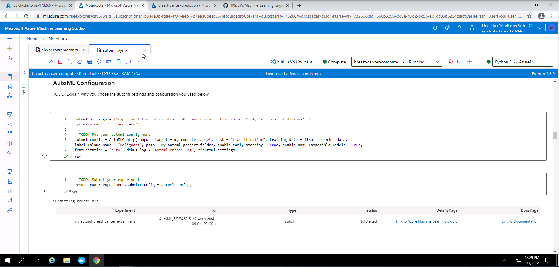
Screenshot 4: Automl setting, configuration and run submission.
Screenshot 4 taken from the notebook shows the AutoML settings and configuration chosen.
AutoML setting Seting details Value used experiment_timeout_minutes Experiment duration in minutes 30 max_concurrent_iterations Maximum nuber of iterations that will be executed in parallel 4 n_cross_validations The number of cross validations to perform 5 primary_metric The primary metric that will be optomized to find the best model "accuracy" AutoML configuration Config details Value used compute_target The compute target that will be used to run the experiment bc-compute task type of task that AutoML will run "classification" training_data Dataset that will be used to train the models final_training_dataset label_column_name The column that will be used as the predicted outcome "malignant" path Path to my project folder my_automl_project_folder enable_early_stopping Method to stop training if the accuracy does not improve True enable_onnx_compatible_models Enable or disable the use of onnx compatible models True featurization Choice of featurization to be used "auto" debug_log Choose a name for the AutoML error/debug log "automl_errors.log" 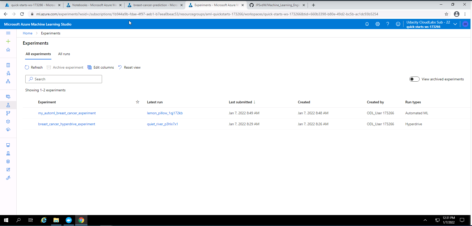
Screenshot 5: List of experiments.
screenshot 5 shows a list of experiments the focus here is on "my_automl_breat_cancer_experiment. This list can be found under the experiments section in Azure Machine Learning Studio.
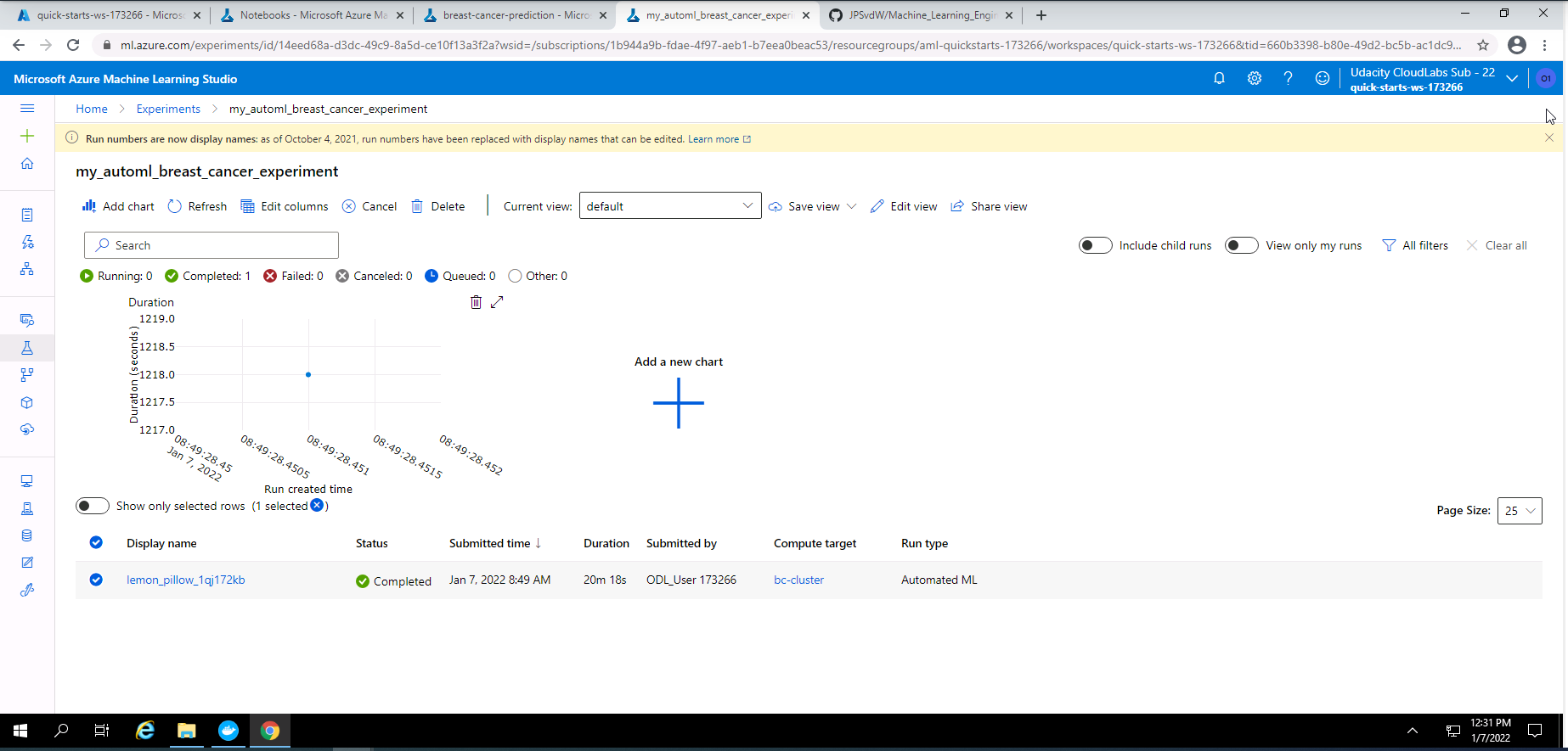
Screenshot 6: AutoML experiment.
Screenshot 6 shows that my AutoML experiment has completed successfully. This screenshot can be found by clicking on "my_automl_breast_cancer experiment" under the experiments section of Azure Machine Learning Studio.

Screenshot 7: Details of the AutoML experiment.
Screenshot 7 provides high level details on the completed AutoML experiment. This screenshot was accessed by clicking on lemon_pillow_1qj172kb at the bottom of screenshot 6.
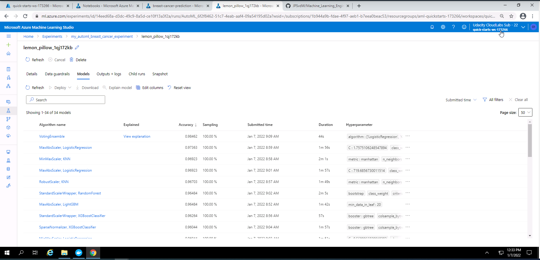
Screenshot 8: Models pruduced by the AutoML experiment.
Screenshot 8 provides a list of the models trained during the AutoML experiment. This screen was accessed under Models tab from screenshot 7.
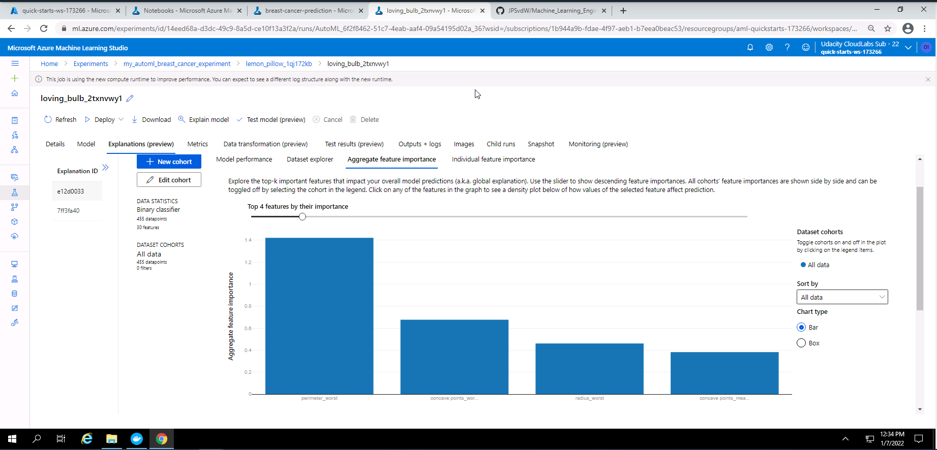
Screenshot 9: Explanation of the best model (VotingEnsemble).
screenshot 9 provides an explanation of the best model from the AutoML experiment which is a Voting Ensemble model. The explanation in this screenshot provides the top four important features used in the training of this model. This screen can be accessed by clicking on the explanation link next to the best model (VotingEnsemble) in screenshot 8.
-
Show run details by using the run details widget.
-
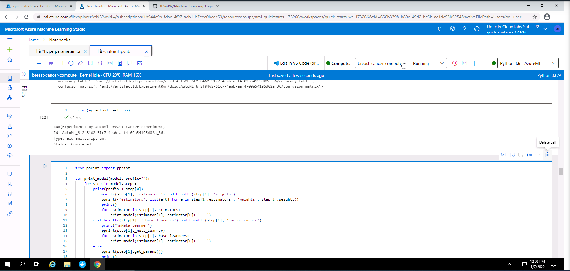
Display the details of the best model.
-
Save and register the best model.
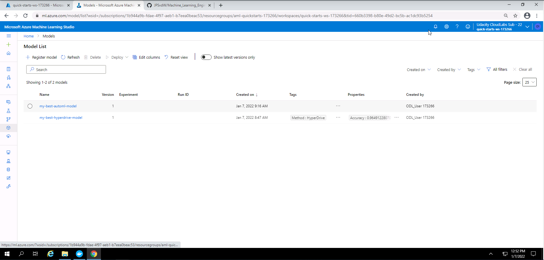
Screenshot 10: List of registered models.
Screenshot 10 provides a list of the best models that was registered. In this section we only focuss on the best AutoML model that was registered. This screen was accessed under the models section.
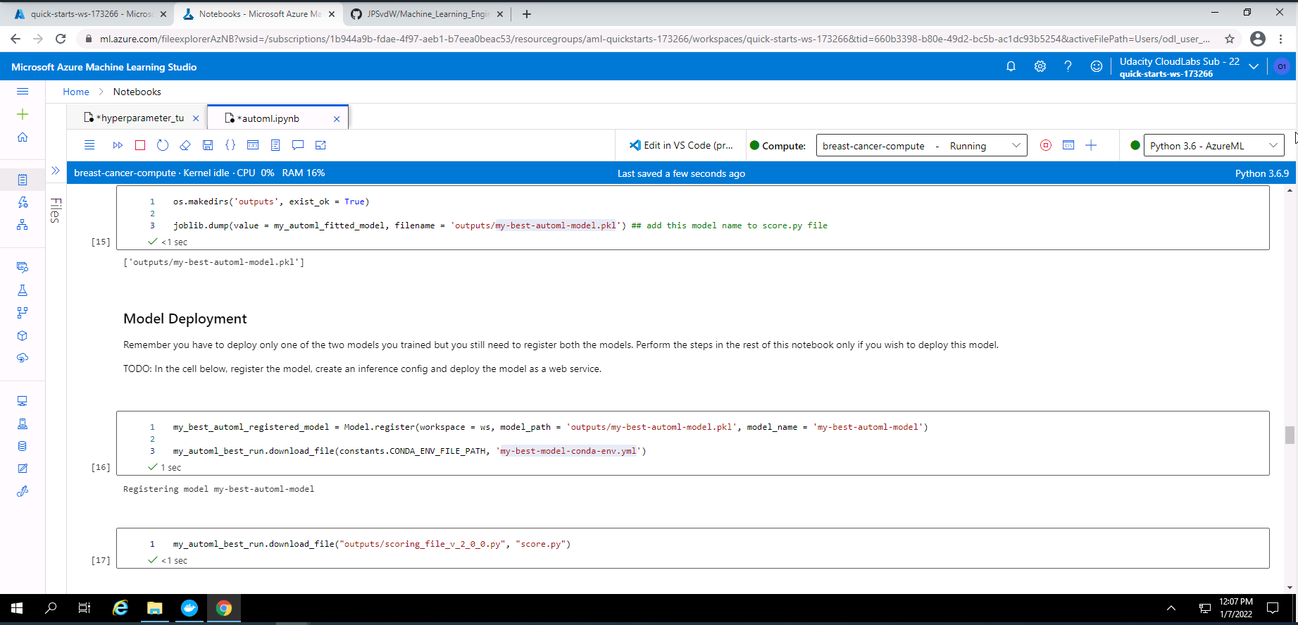
Screenshot 11: Model registartion in Notebook.
Screenshot 11 provides confirmation that I have registered the best AutoML model using code in a Jupyter Notebook.
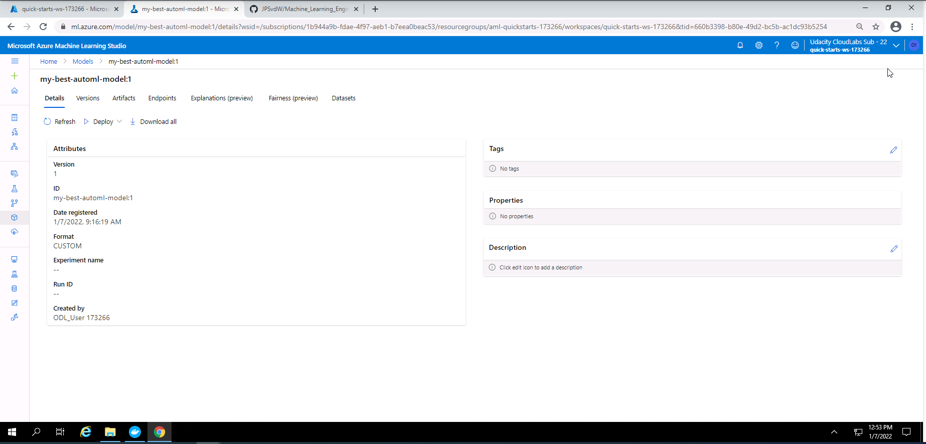
Screenshot 12: Details of the best AutoML model that was registered.
Screenshot 12 provides confirmation that I successfully registered the best AutoML model. This screenshot specifically show some high level details of the AutoML models that was registered. This screenshot was accessed by clicking on "my-best-automl-model" in screenshot 10.
- Deploy the best model as an Azure Container Instance (ACI).
- Show the state of the deployed model.
- Send a request to the deployed model and obtain a prediction.
- print web service logs.
- Convert and save the best model to a onnx format.
- Delete the service.
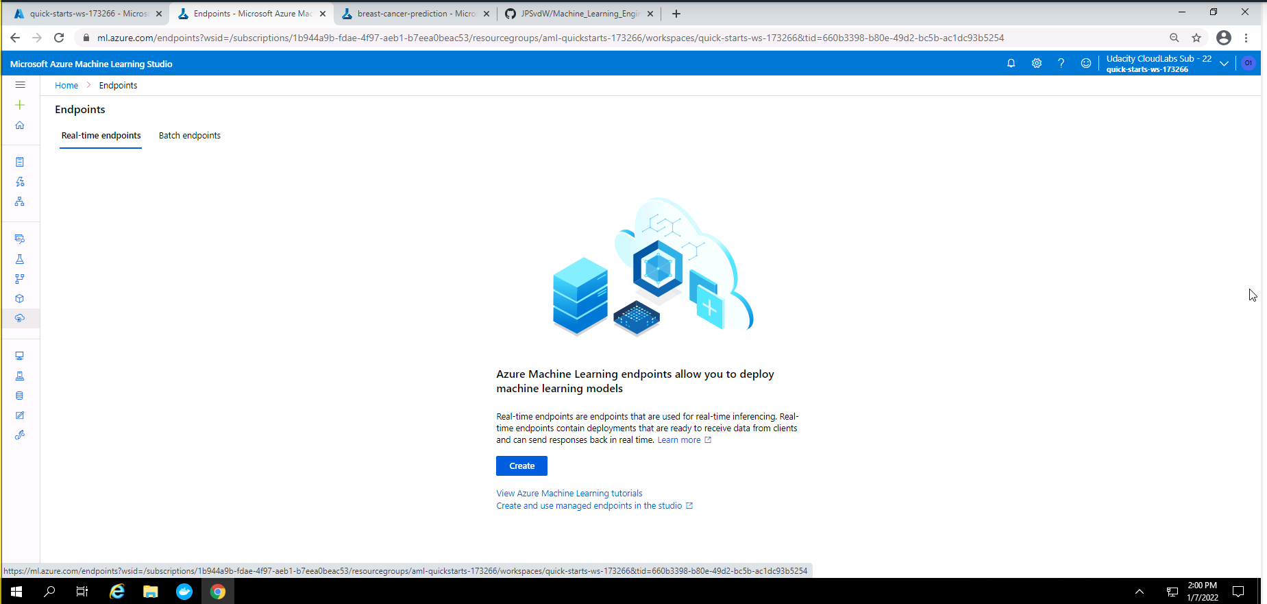
Screenshot 12: Proof that services was deleted.
Screenshot 12 provides proof that all services used in this project was deleted. This screenshot was accessed under the endpoints section.
The results from the AutoML experiment were as follow:
- Best model = Voting Ensemble
- Accuracy = ~ 98%
Screenshot 13: RunDetails widget with list of models.
Screenshot 13 shows the RunDetails widget with a list of the completed models. This screenshot was taken from my Notebook after the execution of the code for the RunDetails widget.
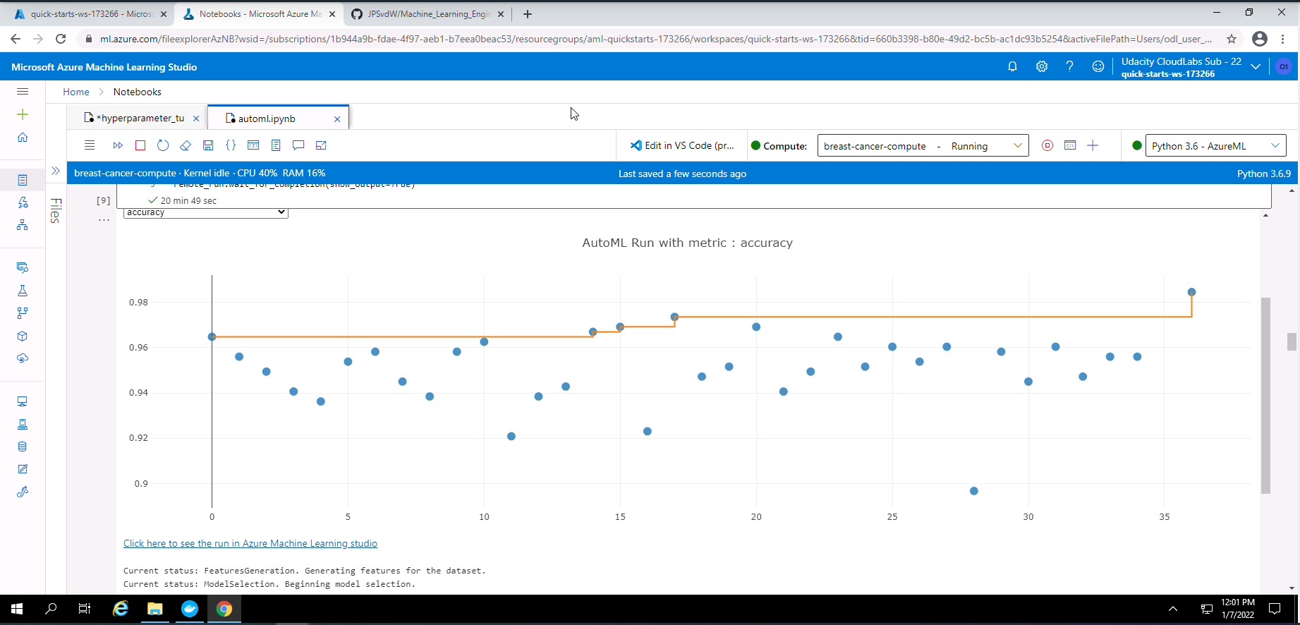
Screenshot 14: RunDetails widget with a graph of the accuracy of the models.
Screenshot 14 shows the RunDetails widget with a graph of the accuracies of the completed models. This screenshot was taken from my Notebook after the execution of the code for the RunDetails widget.
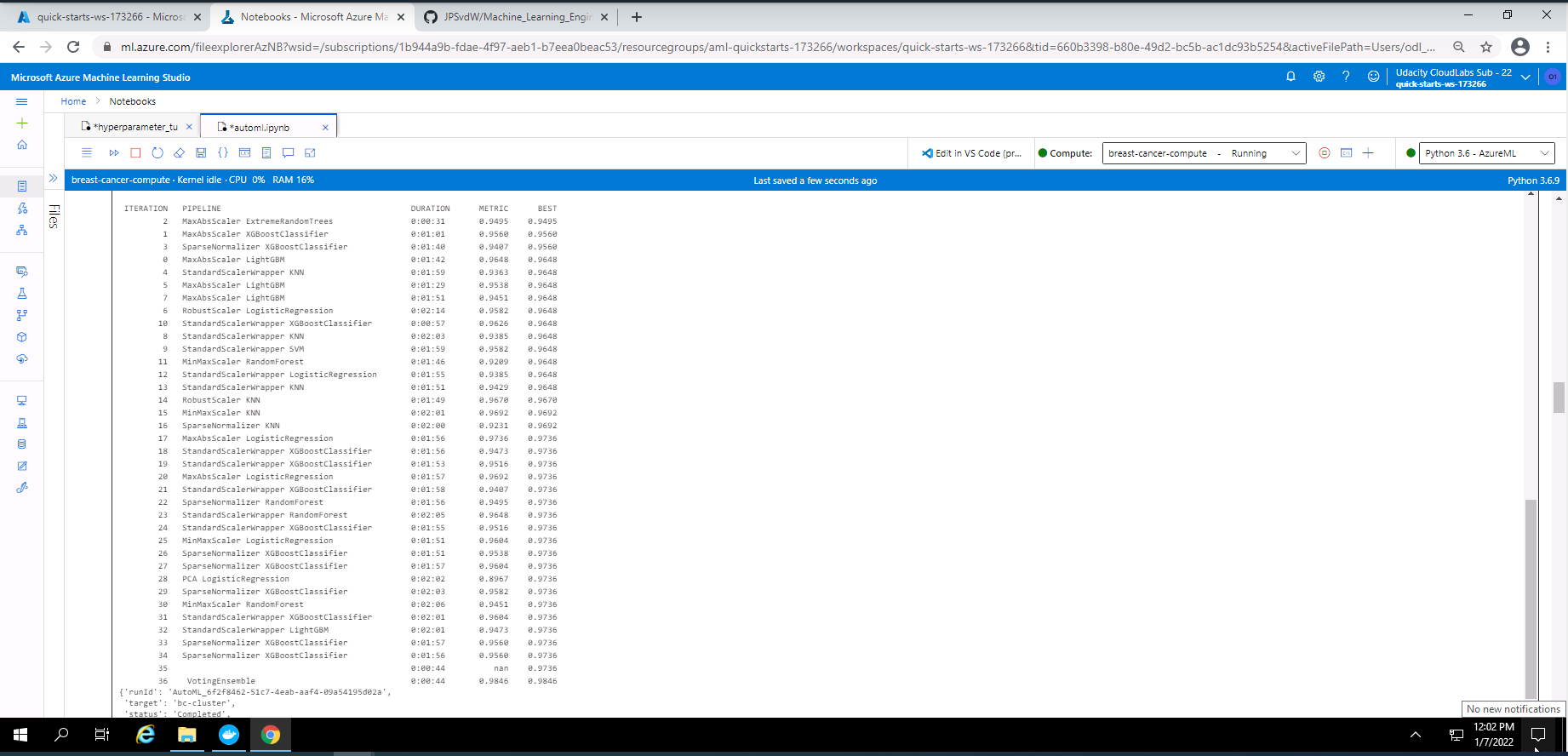
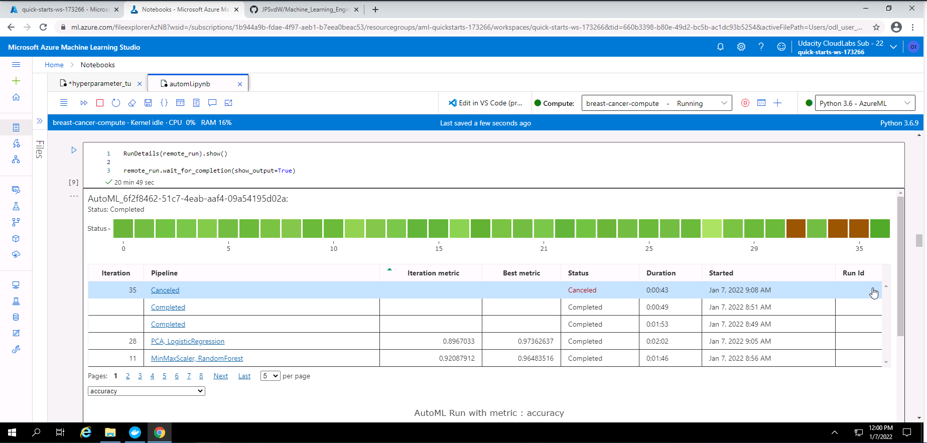
Screenshot 15: List of all the models trained.
Screenshot 15 shows a list of all the models trained by the AutoML experiment. The duration of training and the metric is provided next to each model.
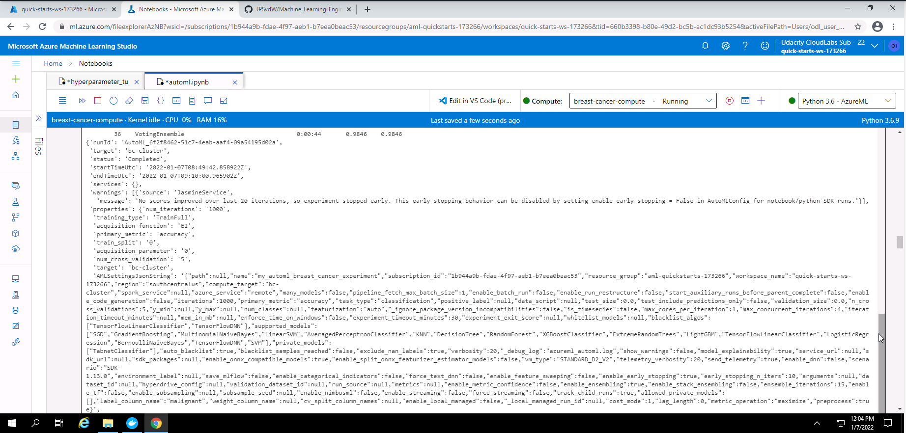
Screenshot 16: Output from the AutoML experiment.
Screenshot 16 provides some output regarding the AutoML experiment that was completed successfully.
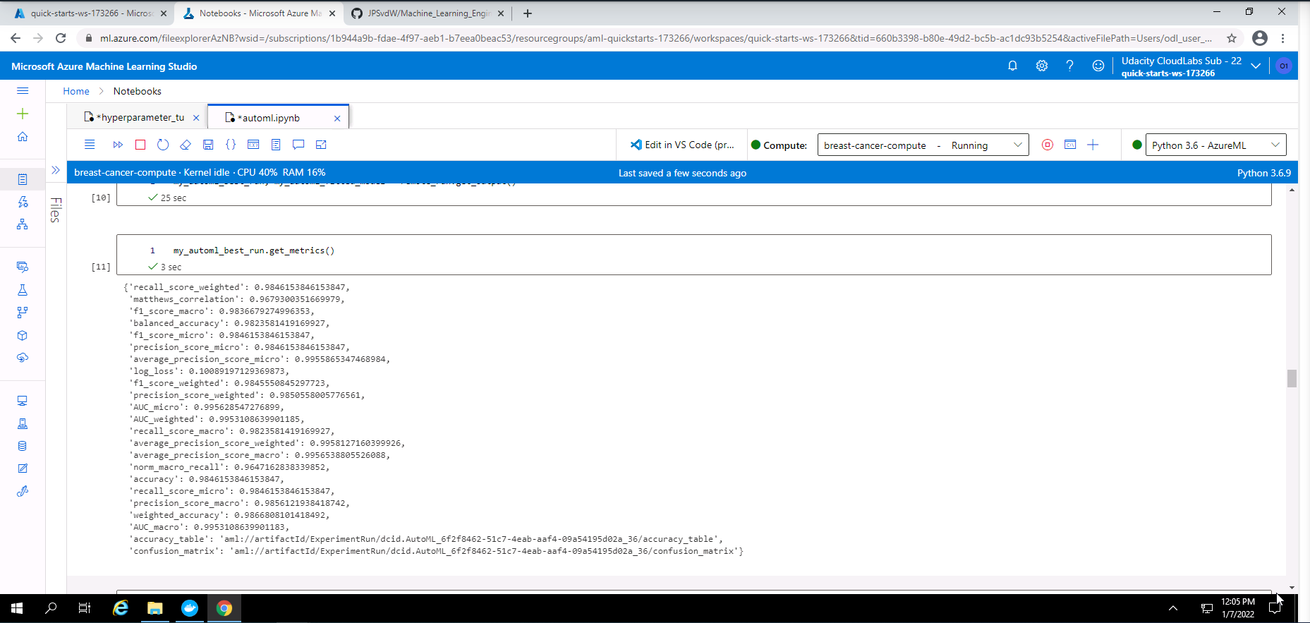
Screenshot 17: Metrics of the best AutoML model.
Screenshot 17 provides all of the metrics for the best AutoML model.
Screenshot 18: Details of the best AutoML model.
Screenshot 18 provides details of the best AutoML model. Details like "Run ID", "Type" and "Status" is shown.
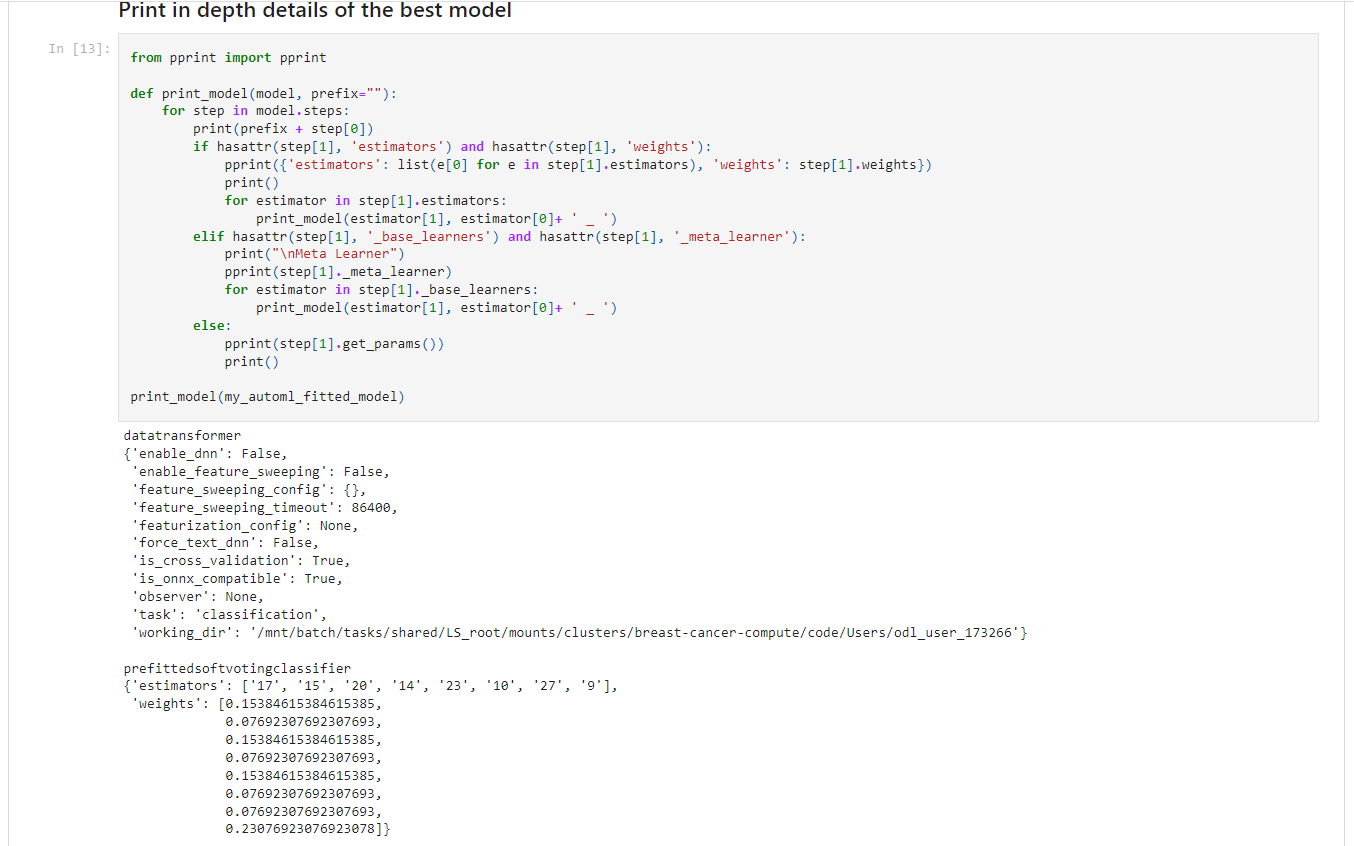
Screenshot 19: Parameters of the trained Voting Ensemble model.
Screenshot 19 provides a view of the parametrs from the best AutoML model (VotingEnsemble) that was trained during the experiment. To llok at the complete output of parameters, please look at the "ensemble_model_parameters.txt" file in this repository.
| Algorithm | Wheight |
|---|---|
| logisticregression - maxabsscaler ('C': 1.7575106248547894) | 0.15384615384615385 |
| kneighborsclassifier - minmaxscaler | 0.07692307692307693 |
| logisticregression - maxabsscaler ('C': 719.6856730011514) | 0.15384615384615385 |
| kneighborsclassifier - robustscaler | 0.07692307692307693 |
| randomforestclassifier - standardscalerwrapper | 0.15384615384615385 |
| xgboostclassifier - standardscalerwrapper | 0.07692307692307693 |
| xgboostclassifier - sparsenormalizer | 0.07692307692307693 |
| svcwrapper - standardscalerwrapper | 0.23076923076923078 |
A Voting Ensemble model combines the outputs of multiple algorithms. The final model consists of a wheighted sum of all the chosen algorithms' outputs.
The accuracy of the model could be improved by increasing the experimant duration. This would give increase training time which might lead to better model accuracy. If a medical practitioner has in depth knowledge it can help to do specific feature engineering and provide those specific features rather that allowing AutoML to automate it. This could also possibly improve the accuracy of the final model.
I chose to use a logistic regression model to predict wheter the tissue from a breast tumor is benign or malignant. I chose this model due to its simplicity with regards to implementation and interpretation, and low computational needs. I have chosen to optimize the following two parameters:
- Regularization strength C with uniform search space of (0.1, 1)
- maximum iteration with a choice of (50, 100, 150, 200, 250)
I chose a random parameter sampling method due to it saving computational resources. Although this sampling method saves on computational resources it still produces reasonably good models. Sampling methods like Grid Parameter Sampling, will use every value within a search space thus using significantly more computational resources. The Random Parameter Sampling method also allows for early termination policies. This allows for the termination of runs performing poorly.
I chose an early termination policy called BanditPolicy. This is one of the more aggressive policies, allowing to stop more runs. This type of early termination policy results in significat reduction of computation time. The following parameters were used in the BanditPolicy:
- evaluation_interval = 1, this is the frequency at which the policy will be applied.
- slack_factor = 0.1, this is the amount of slack between a executing run and the best performing training run.
- delay_evaluation = 4, number of interval to delay the policy and avoids premature termination.
In this section i executed a number of code cells from my "hyperparameter_tuning.ipynb" Notebook. The following is an overview of steps executed in this notebook:
- Import all dependencies.
- Load, show first few lines of the dataset, and statistics.
- Choose an experiment name.
- Create a AML Compute Cluster or reuse if already exists.
Screenshot 20: re-use AML compute cluster created.
Screenshot 20 provides confirmation that the AML compute cluster was created successfully. This cluster will be re-used in this section.
- Add Hyperdrive configuration and settings.
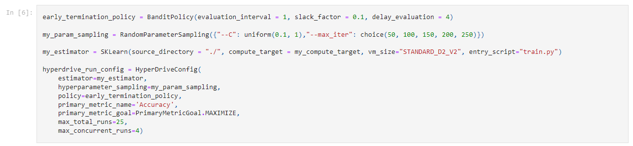
Screenshot 21: Hyperdrive settings and configuration.
Screenshot 21 shows the Hyperdrive settings and configuration chosen.
- Submit experiment.
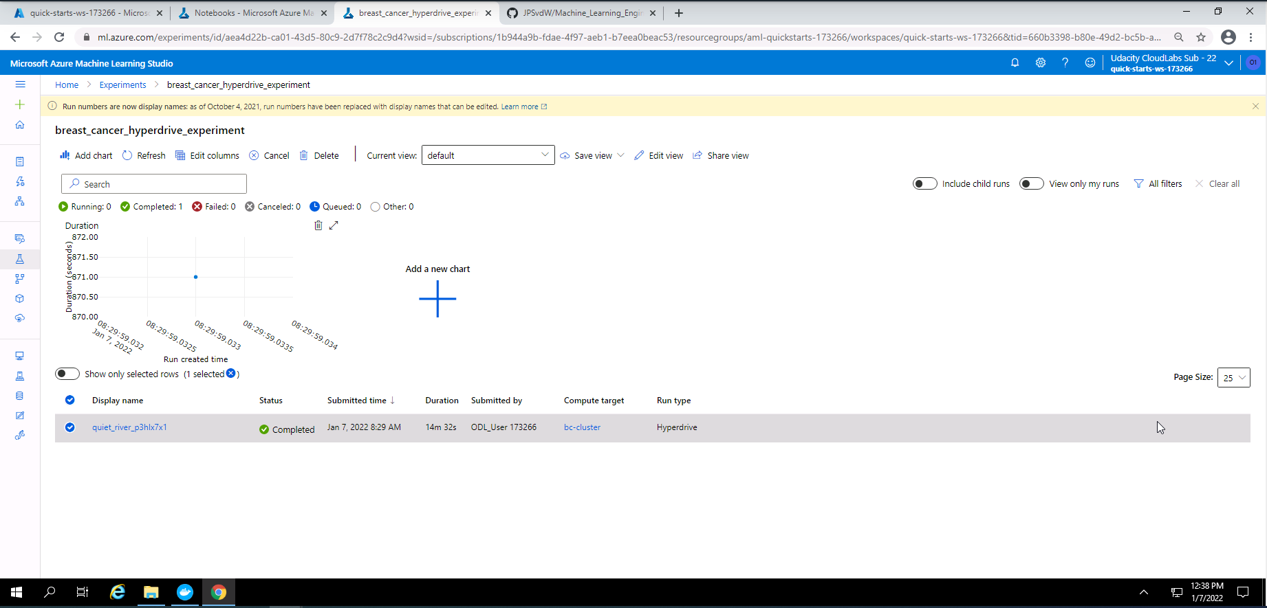
Screenshot 22: Completed Hyperdrive experiment.
Screenshot 22 provides confirmation that my Hyperdrive experiment has completed successfully. This screenshot wass accessed under the experiments tab and clicking on "breast_cancer_hyperdrive_experiment".
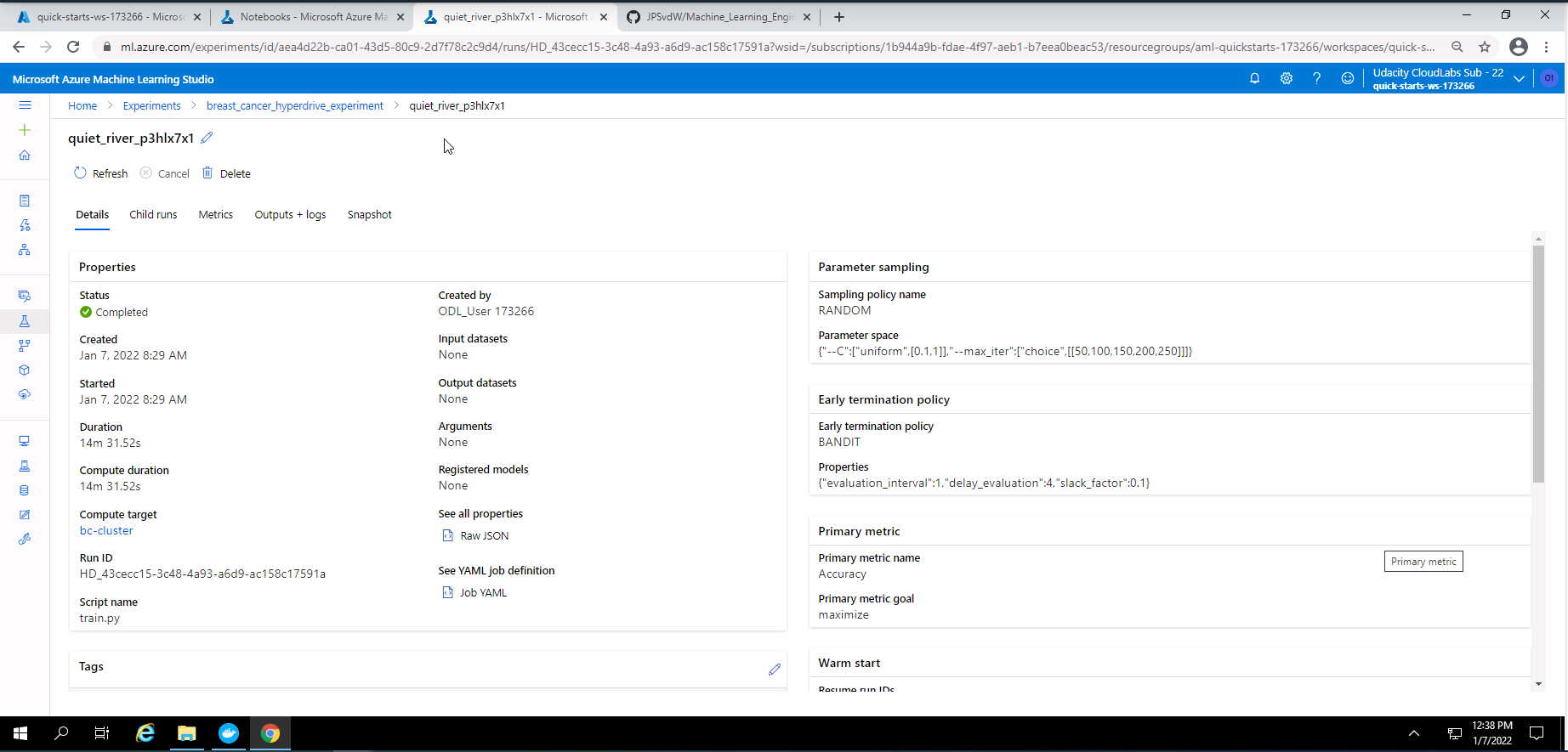
Screenshot 23: Hyperdrive experiment details.
Screenshot 23 provides some details on the best Hyperdrive model. The screenshot was accessed by clicking on "quiet_river_p3hlx7x1" at the bottom of screenshot 22.
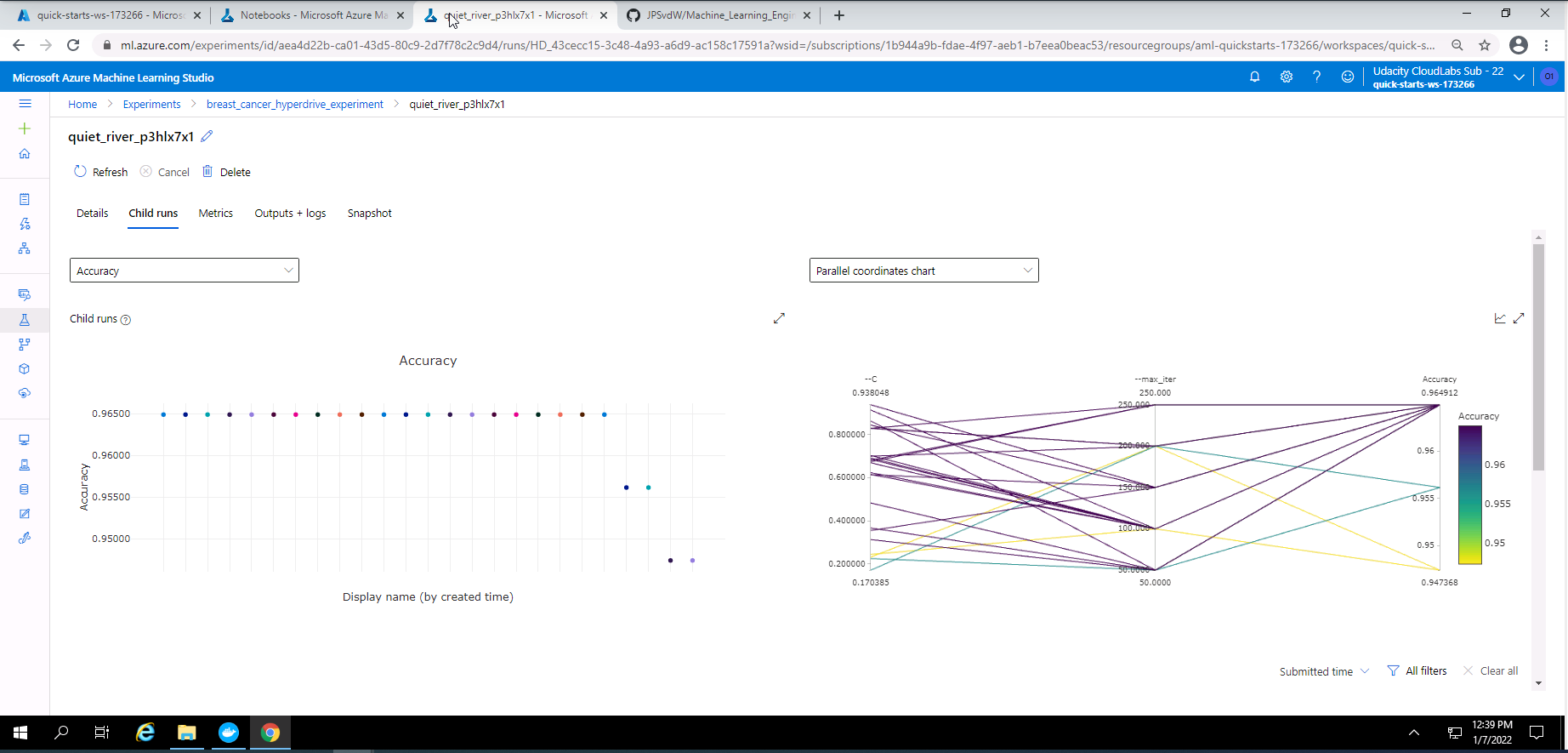
Screenshot 24: Hyperdrive experiment child runs.
Screenshot 24 provides a visual view of the child runs completed during the Hyperdrive experiment. This screen can be accessed under the child runs tab in screenshot 23.
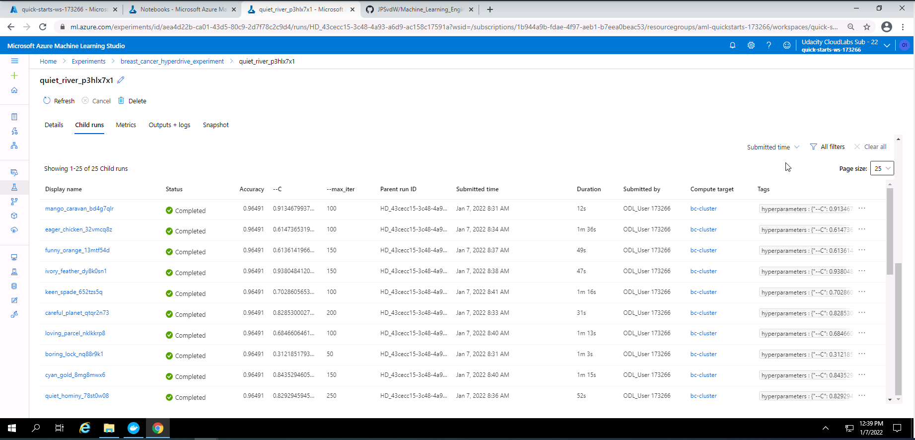
Screenshot 25: List of child runs.
Screenshot 25 shows the list of child runs completed. This screen is shown when scrolling dow in screenshot 24.
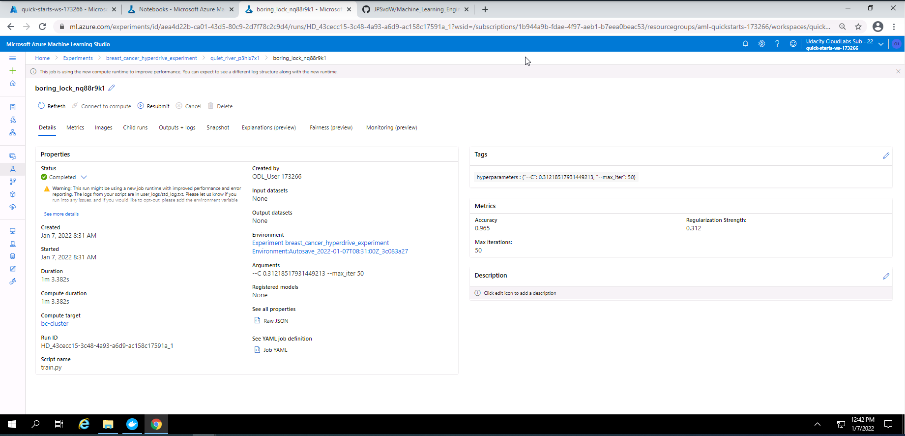
Screenshot 26: Details of the best Hyperdrive run.
Screenshot 26 provides details on the best Hyperdrive run.
- Show RunDetails using widget.
- Provide details on the best Hyperdrive model.
- Save and register the best hyperdrive model.
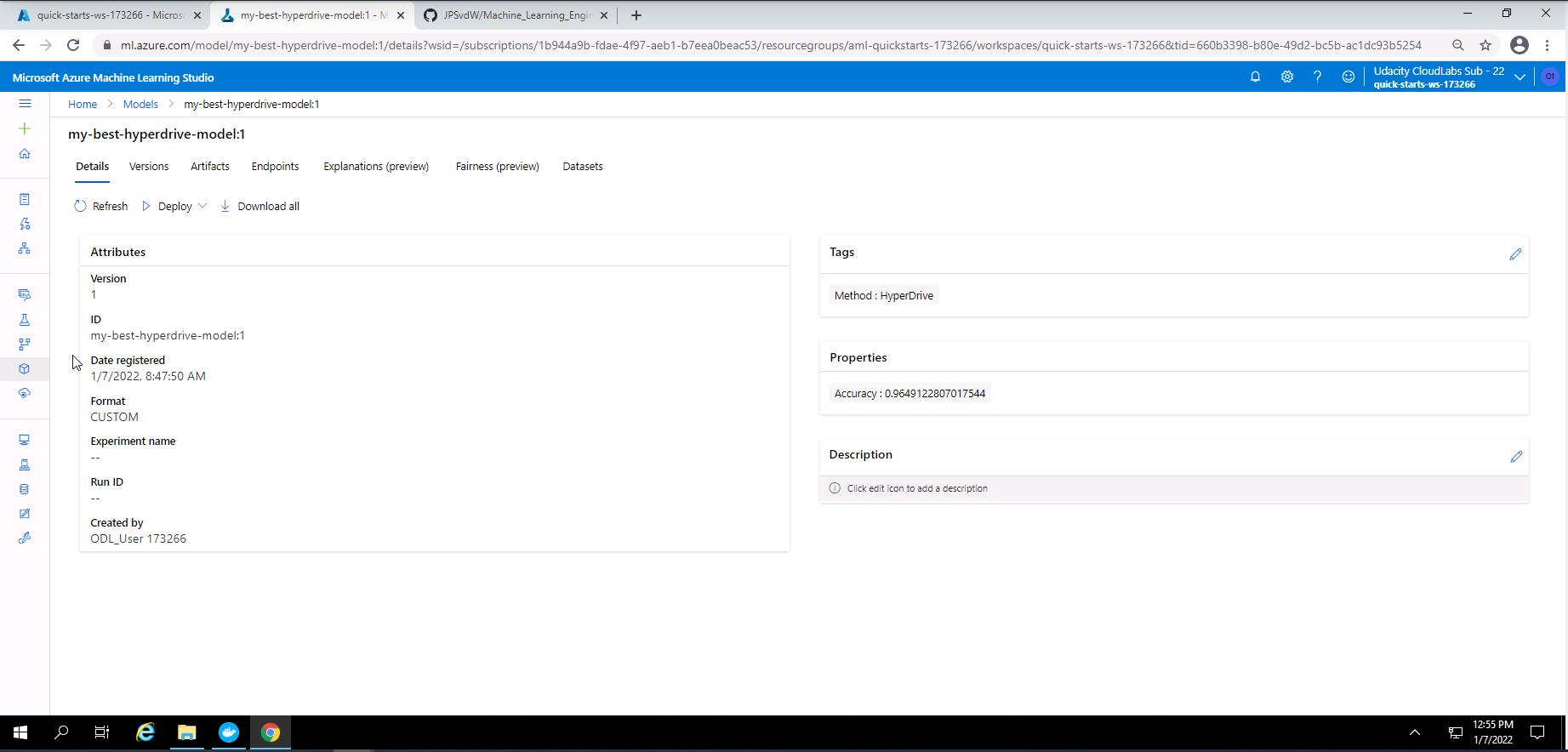
Screenshot 27: Details of the best hyperdrive model.
Screenshot 27 shows an overview of the details from the best Hyperdrive model that was registered in Azure Machine Learning Studio.
The best hyperdrive model had an accuracy of approximately 96%. The hyperparameter values for this model:
- Regularization strength of 0.31218517931449213
- Maximum iteration of 50
One way to improve the accuracy of this model is to take the regularization strength value and maximum iteration from this model and refine it with a Grid Parameter Sampling method.
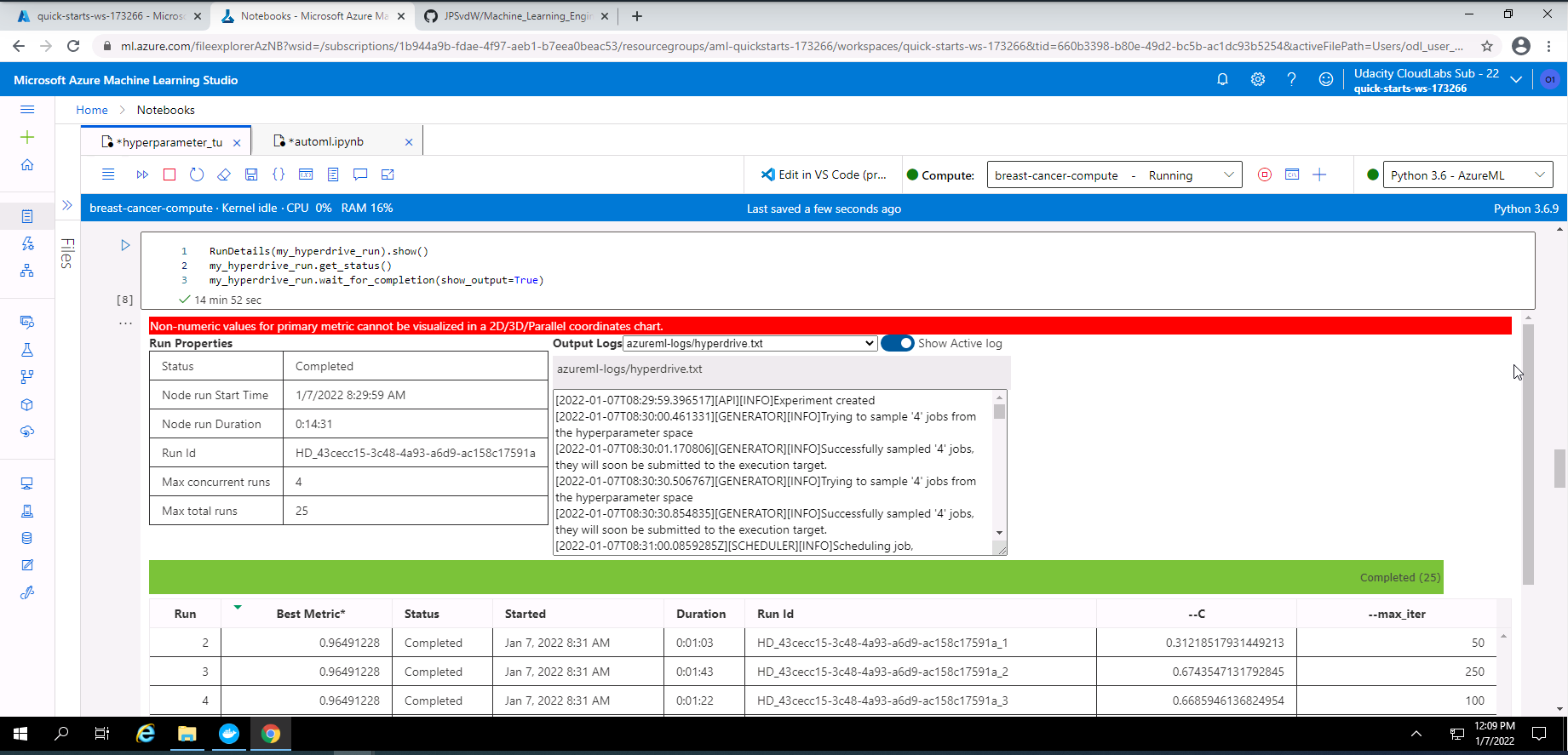
Screenshot 28: RunDetails widget with run list.
Screenshot 28 provides the completed run list of the Hyperdrive experiment.
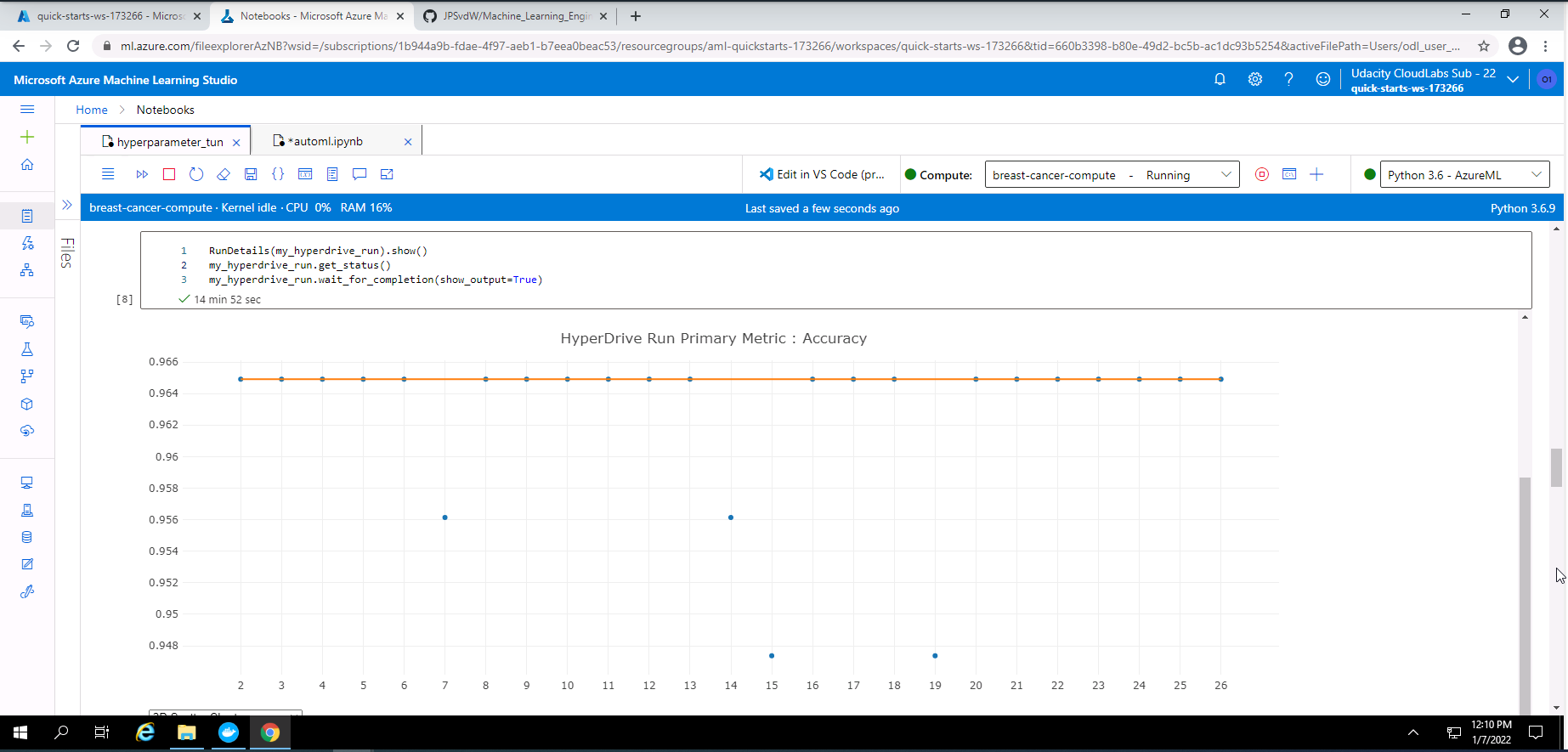
Screenshot 29: RunDetials widget showing graph of run accuracies.
Screenshot 29 provides a graph of the accuracy for each completed run.
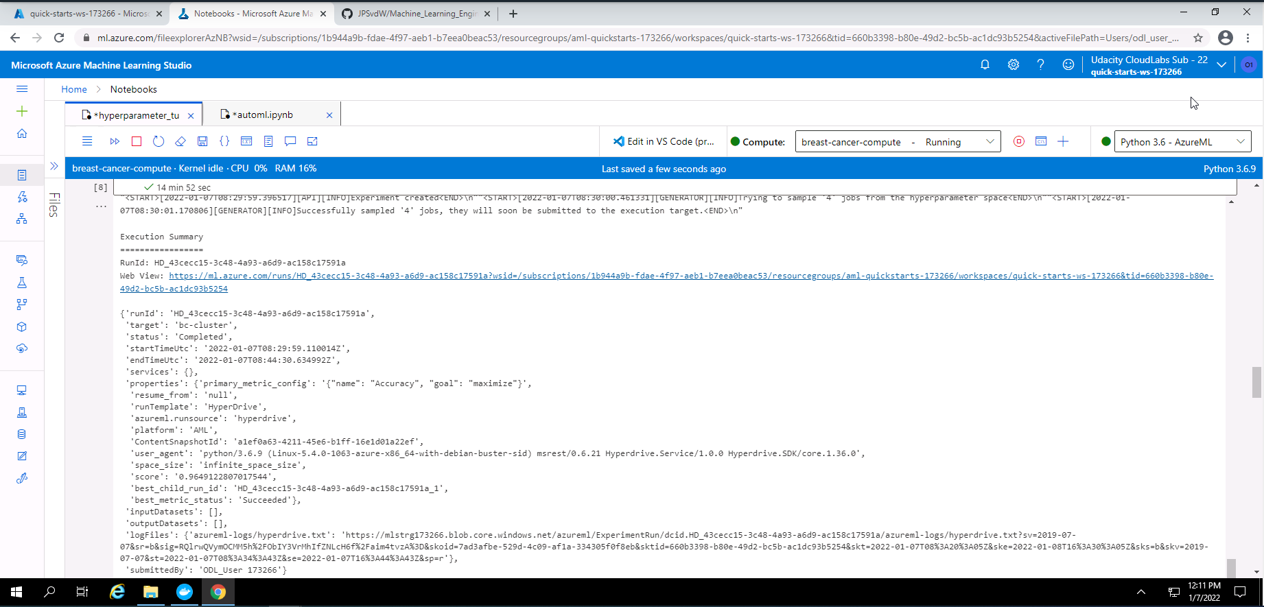
Screenshot 30: Hyperdrive experiment output.
Screenshot 30 provides a text based output of the completed Hyperdrive experiment.
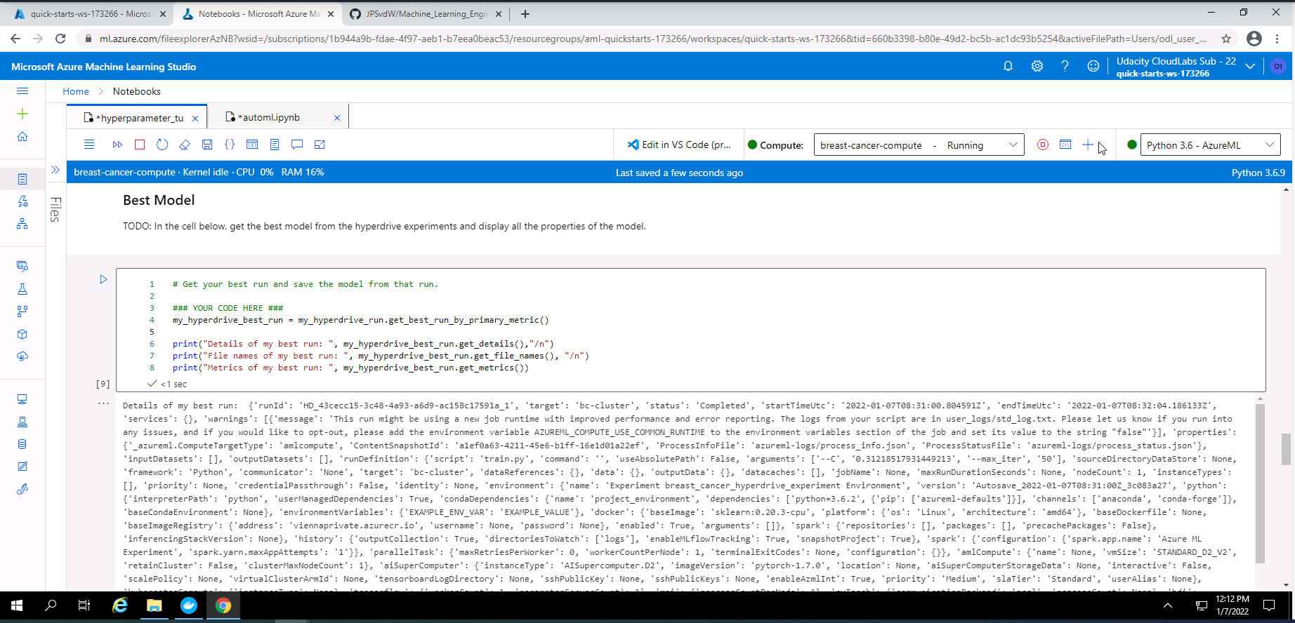
Screenshot 31: Detailed information from the best Hyperdrive model.
Screenshot 31 provides in depth information regarding the best model from the Hyperdrive experiment.
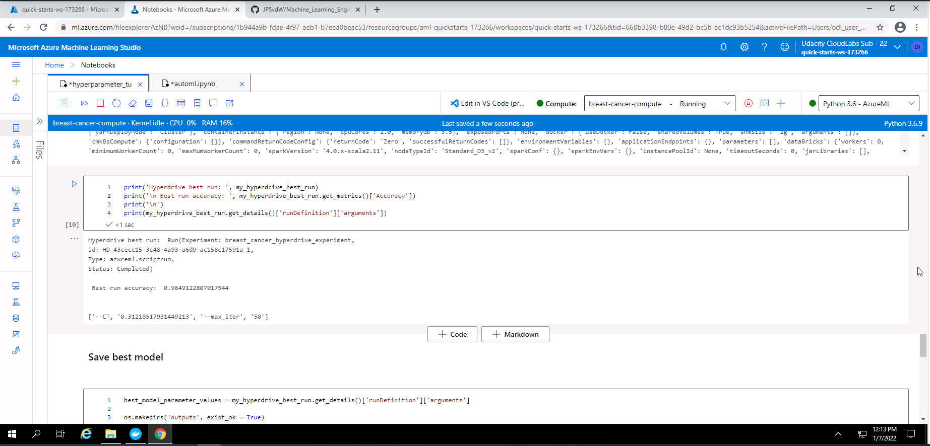
Screenshot 32: Summary of the best Hyperdrive model.
Screenshot 32 provides a summary of the best Hyperdrive model. The run Id, status, best run accuracy of ~96%, and the hyperparameter values of the best model is shown.
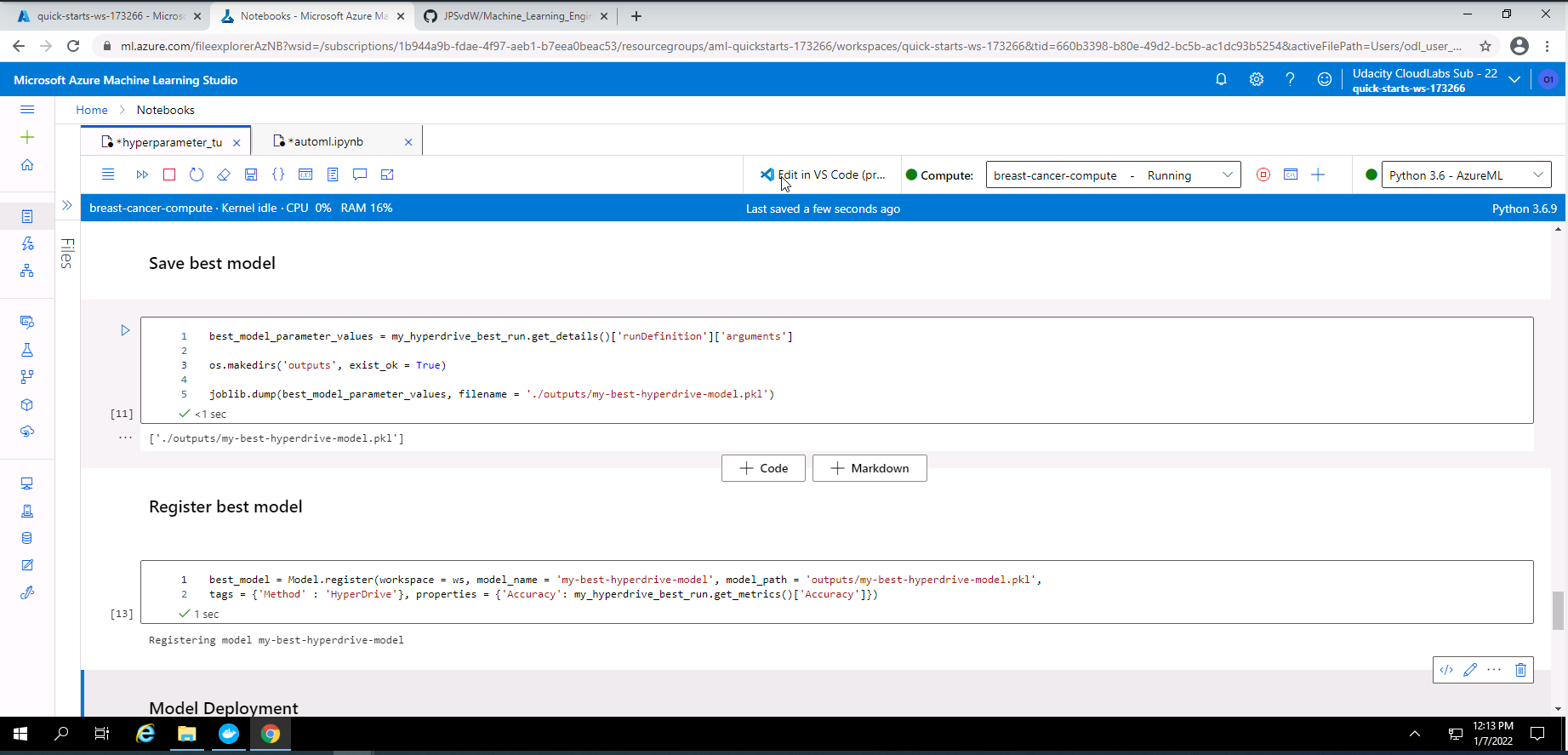
Screenshot 33: Save and register model.
Screenshot 33 provides confirmation that the best Hyperdrive model has been saved and registered.
The model with the best accuracy of approximately 98% and was obtained from the AutoML experiment. The Hyperdrive model had a accuracy of approximately 96%. Therefore I will deploy the best model from the AutoML experiment.
In order to deploy this model, I had to navigate to the outputs and logs section of the best AutoML model and download and save my environment variables file and scoring python file that was generated by AutoML. These two files can be found in this repository with the names "my-best-model-conda-env.yml" and "score.py".
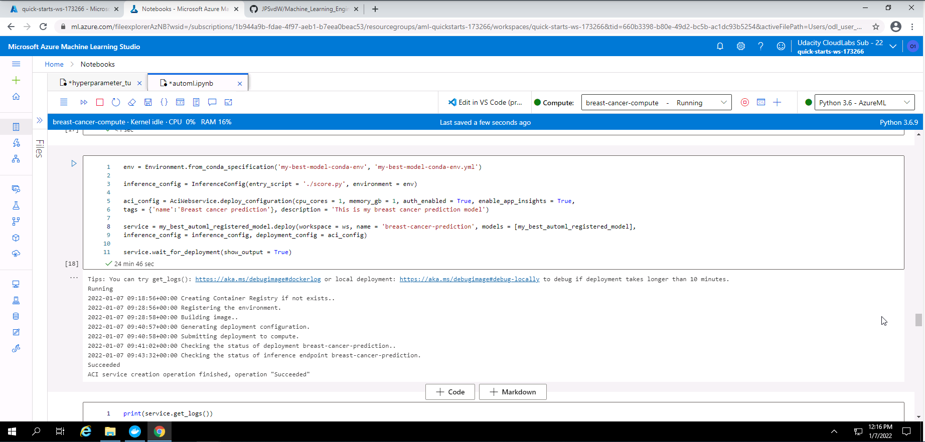
Screenshot 34: Model deployement set-up.
From screenshot 34, it is seen that I pass the environment details file and score.py file to the inference config method. I used an Azure Container Instance Webservice deployment with one CPU core, 1GB of memory, enabled authentication, and enabled application insights. From the output in this screenshot, it is observed that the deployment was successful.
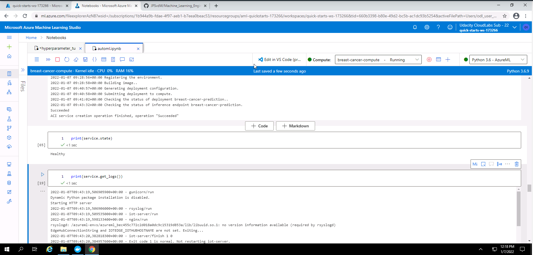
Screenshot 35: Model deployment status.
From screenshot 35 it is seen that the deployment state is healthy. It is also seen that the model logs are also showing.
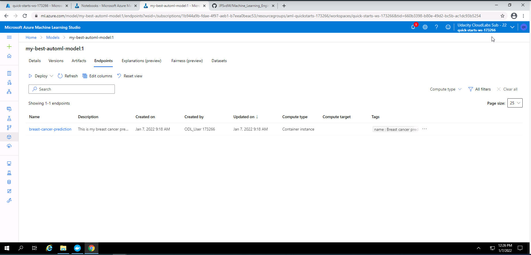
Screenshot 36: Deployed model endpoint.
Screenshot 36 was taken from the endpoints section in Azure Machine Learning Studio and lists the deployed model endpoint.
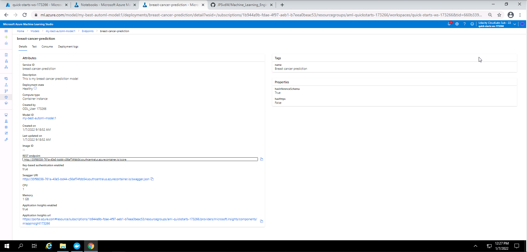
Screenshot 37: Deployed endpoint details.
Screenshot 37 provides the details of the deployed endpoint and can be found when clicking on the endpoint in screenshot 36. In this screenshot it can be seen that the deployment state is healthy, authentication is enabled and application insights is also enabled. The resp endpoint and swagger URI is also provided.
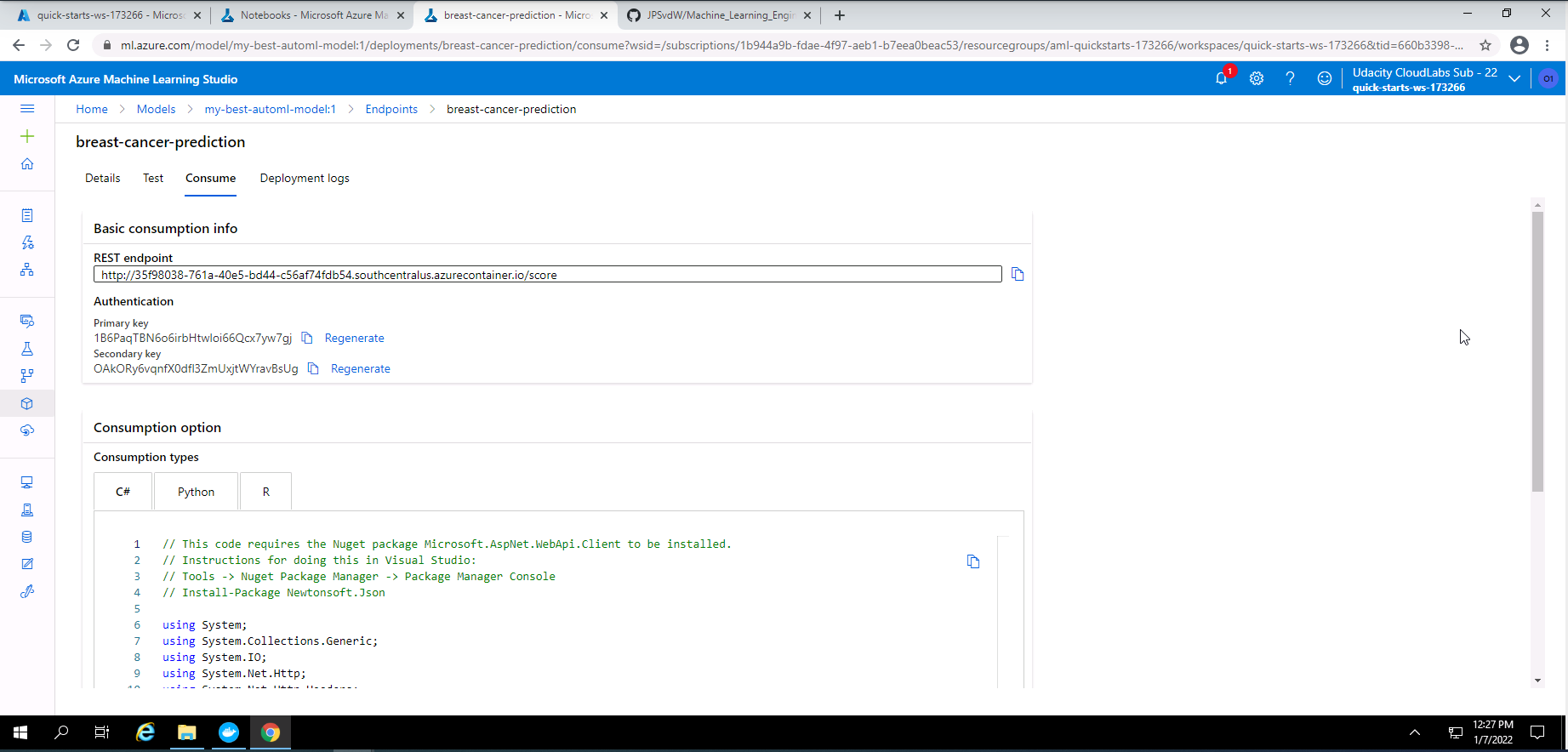
Screenshot 38: Endpoint consume tab.
Screenshot 38 shows the consume tab of the deployed model endpoint. From here we can get the REST endpoint address and also the authentication keys.
The folowing is the code used to interact with the deployed model rest endpoint.
import requests
import json

scoringuri = service.scoring_uri

key = service.get_keys()[0]

#print(scoringuri)
#print(key)

data = {
  "Inputs": {
    "data": [
      {
        "radius_mean": 18.0,
        "texture_mean": 10.40,
        "perimeter_mean": 122.9,
        "area_mean": 1002,
        "smoothness_mean": 0.1185,
        "compactness_mean": 0.2778,
        "concavity_mean": 0.3002,
        "concave points_mean": 0.1473,
        "symmetry_mean": 0.2420,
        "fractal_dimension_mean": 0.07873,
        "radius_se": 1.096,
        "texture_se": 0.9054,
        "perimeter_se": 8.590,
        "area_se": 153.6,
        "smoothness_se": 0.00640,
        "compactness_se": 0.04906,
        "concavity_se": 0.05375,
        "concave points_se": 0.01588,
        "symmetry_se": 0.03004,
        "fractal_dimension_se": 0.006195,
        "radius_worst": 25.40,
        "texture_worst": 17.40,
        "perimeter_worst": 184.8,
        "area_worst": 2020,
        "smoothness_worst": 0.1625,
        "compactness_worst": 0.6658,
        "concavity_worst": 0.7120,
        "concave points_worst": 0.2656,
        "symmetry_worst": 0.4603,
        "fractal_dimension_worst": 0.1190
      },
      {
        "radius_mean": 13.56,
        "texture_mean": 14.37,
        "perimeter_mean": 87.50,
        "area_mean": 567.0,
        "smoothness_mean": 0.09778,
        "compactness_mean": 0.08130,
        "concavity_mean": 0.06666,
        "concave points_mean": 0.04783,
        "symmetry_mean": 0.1886,
        "fractal_dimension_mean": 0.05768,
        "radius_se": 0.2700,
        "texture_se": 0.7888,
        "perimeter_se": 2.060,
        "area_se": 24.0,
        "smoothness_se": 0.008470,
        "compactness_se": 0.0147,
        "concavity_se": 0.02388,
        "concave points_se": 0.01316,
        "symmetry_se": 0.0199,
        "fractal_dimension_se": 0.0024,
        "radius_worst": 15.12,
        "texture_worst": 19.30,
        "perimeter_worst": 99.9,
        "area_worst": 712.0,
        "smoothness_worst": 0.145,
        "compactness_worst": 0.1775,
        "concavity_worst": 0.240,
        "concave points_worst": 0.1289,
        "symmetry_worst": 0.2979,
        "fractal_dimension_worst": 0.07260
      }
    ]
  },
  "method": "predict"
}
input_data = json.dumps(data)
#print(input_data)
with open("data.json", "w") as _f:
    _f.write(input_data)


headers = {"Content-Type": "application/json"}
headers["Authorization"] = f"Bearer {key}"

response = requests.post(scoringuri, input_data, headers=headers)
print(response.json())
This code stores the deployed model scoring uri, stores the primary key, stores two sampole inputs for scoring, creates a header which sets the content typ to applicatio/json and authorization with Bearer token, and finaly it posts the request.
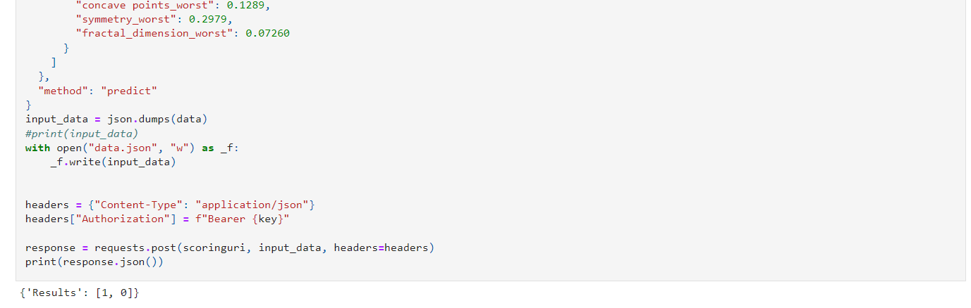
Screenshot 39: Output of the request sent.
Screenshot 39 provides the output of the scoring request. The first sample input returned a prediction of 1 which is malignant and the second sample returned a 0 which is benign.
Although the accuracy of the models in this project are quite good. Some improvements can be done to increase the accuracy of the models. On suggestion could be to introduce nearal networks. Neural networks tend to extract more dependencies between feature and could lead to more accurate models. Another suggestion could be to look at metric other than accuracy. By looking at other metrics a machine learning engineer can ensure that his machine learning model is optimally trained without under fitting or over fitting.
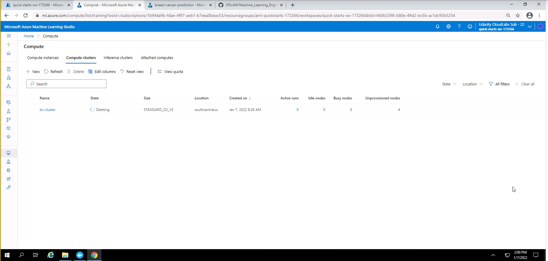
Screenshot 40: Deleting Compute cluster.
Screenshot 40 provides confirmation that the compute cluster has been deleted.
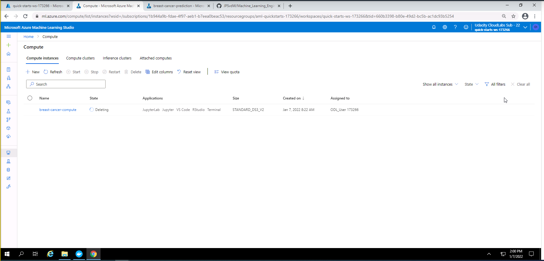
Screenshot 41: Deleting Compute instance.
Screenshot 41 provides confirmation that the compute instance has been deleted.
A screen recording of this project can be accessed by this link.
I decided to convert my best model from the AutoML experiment to a ONNX format as a standout suggestion.
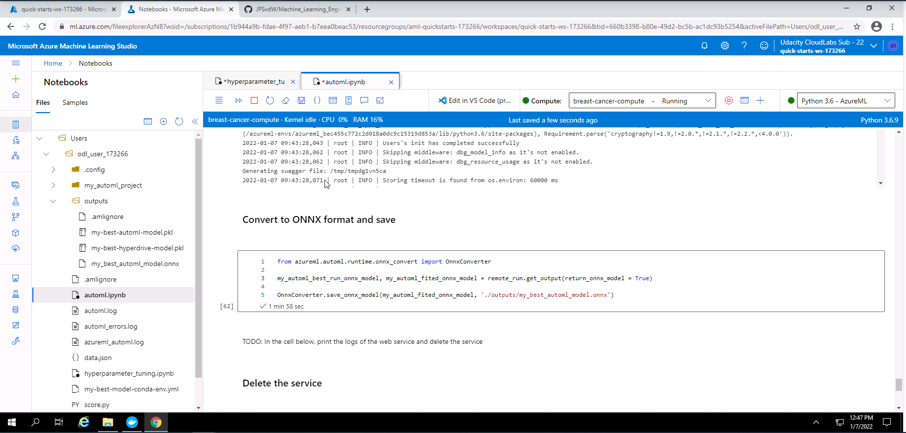
Screenshot 42: Converting model to ONNX format.
Screenshot 42 provides confirmation that I have converted my mydel with the best accuracy to a ONNX format.