This is the second project for the Udacity Machine Learning Engineer with Microsoft Azure Nanodegree Program and relates to the operationalization of machine learning.
In this project I have imported and registerred a bank marketing dataset used to train a classification machine learning model using Automated Machine Learning in Azure Machine Learning Studio. After the AutoML experiment finished the best model (VotingEnsemble) was chosen to be deployed using a an Azure Container Instance (ACI). Application Insights and logging for the deployed model was enabled. Swagger documentation was created for the deployed model HTTP API. The model REST endpoint was then consumed using the Python SDK. Finally a pipeline was created, published and consumed.

Diagram 1: Architectural diagram.
1). Register the Bank Marketing Dataset in Azure Machine Learning Studio.
2). Create an Automated Machine Learning Experiment by creating a Standard_DS12_v2 compute cluster with minimum nodes of one and maximum nodes of six. Enable explain best model and change exit criterion to one hour and concurrency to one less that the maximum nodes of the compute cluster.
3). Choose the best model from the completed experiment and deploy using an Azure Container Instance and enable authentication.
4). Enable Application Insights and logging for the deployed model to be able to monitor performace and any issues.
5). Create a python server and run the latest Swagger container and consume/interact with the Swagger instance running the documentation for the model HTTP API.
6). Make use of the Python SDK and create a python file that will run against the model HTTP API and produce prediction outputs from the model.
7). Make use of a Jupyter Notebook to create a pipeline to choose the best AutoML model and publish it.
There are a few future improvements that would help to improve the model.
1). Increase the training time. The exit criterion was changed to one hour. This could lead to under training of the model. By increasing training time, it insures that the model is not under trained and will increase the accuracy of the model.
2). Use deep learning. Traditional Classification Machine Learning Algorithms are linear. Deep learning introduces multiple hidden layers of of neurons which adds more complexity and abstraction with each layer being added. Deep learning also extracts features without supervision. This means that a Machine Learning Engineer spends less time specifying to the algorithm which features to use for training. The combination of adding complexity, abstraction, and automated featurization, leads to faster training times and more acurate models in the end.
The first step of this project is authentication. This step could not be completed using the virtual machine provided by this course. I went ahead and skipped to the second step.
The second step in this project is to create an Automated ML Experiment.
In order to create an Automated ML Experiment the following steps were taken.
1). I had to upload and register the bankmarketing_train.csv to Microsoft Azure Machine Learning Studio. The dataset was dowloaded to the computer and was uploaded to Azure Machine Learning Studio using the from local files method.
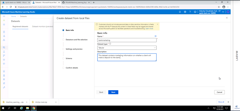
Screenshot 1: Adding details to the dataset being registered.
Screenshot 1 shows the addition of basic information of the dataset being registered. Information like the name of the dataset, dataset type and a description is added.
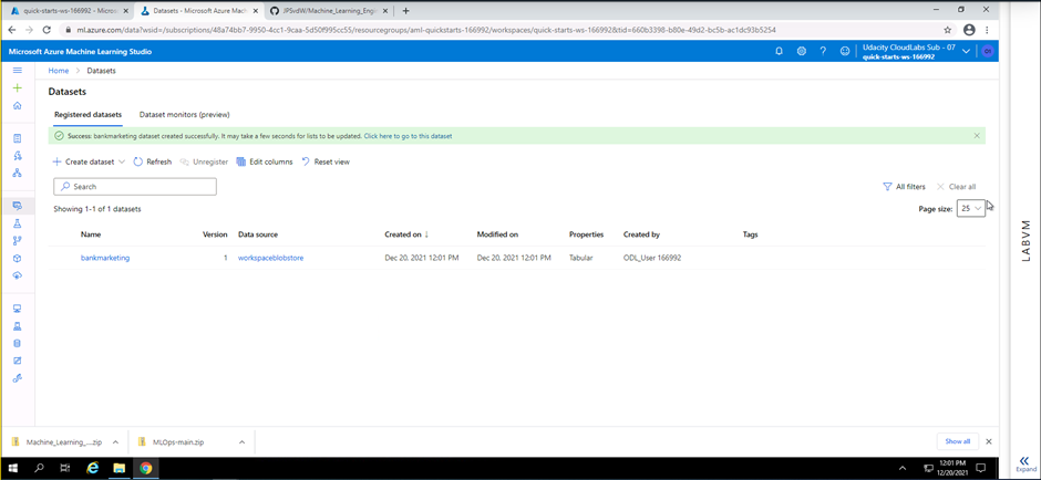
Screenshot 2: Dataset registered
Screenshot 2 privides confirmation that the new sdataset has successfully been registered on Microsof Azure Machine Learning Studio. The screenshot also provides extra details regarding the registered dataset. Information like the name, data source, date created, date modified, properties of the dataset and who created the dataset is shown.
The bankmarketing_train.csv file contains fields pertaining to information gathered during a marketing outreach on whether a client will make a deposit to a bank
2). The second important step to be able to create an Automated ML Experiment is to configure a compute cluster. A standard_DS12_V2 compute cluster with a minimum of one node and a maximum of 6 nodes was created.
3). Now that a dataset has been registered and a compute cluster has been created, an Automated ML run can be created. Thereafter, a automated ML experiment was created. The following configuration was used for the Automated ML Experiment:
- Classification was used to predict the outcome.
- On exit criterion default time was reduced to 1 hour. (This is to reduce the training time due to the Virtual Machine Time limit)
- Concurrency was set to 5, which should always be one less than the maximum nodes specified in the compute cluster.
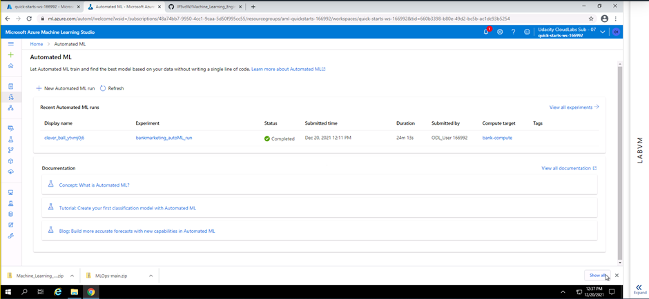
Screenshot 3: Automated ML run complete.
Screenshot 3 provides confirmation that the Automated ML run has completed successfully. Information like the run name, experiment name, status, submitted time, duration, submitted by and compute target used is provided.
The following screenshots will show that the best model from the exiperiment as a Voting Ensemble. This model was then chosen to be used in the steps that will follow.
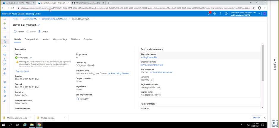
Screenshot 4: Completed Automated ML Experiment.
Screenshot 4 provides confirmation that the Automated Ml experiment has completed successfully. This screenshot provides details of the best trained model produced during this experiment. The best model is a voting ensemble algorithm and has a AUC weighting of 0.94791.
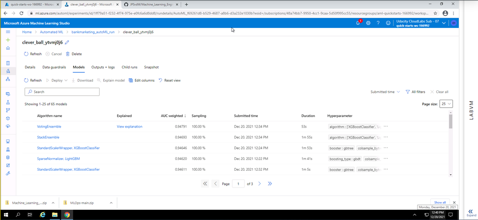
Screenshot 5: List of all models pruduced.
Screenshot 5 provides details on all the models trained during the experiment. This information can be found under the models tab within the Automated ML section. The algorithm name, AUC weighting, sampling and duration for each model is given. Explanation of the best model was enabled and a link to the explanation is provided in the explained column next to the best model (VotingEnsemble).
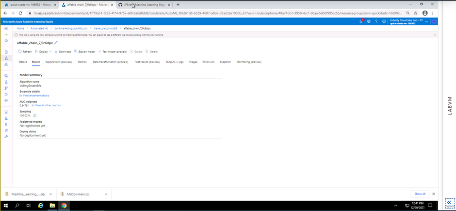
Screenshot 6: Overview of the best model
Screenshot 6 provides a high level view of the best model. In this screenshot the algorith name and AUC weighting can be seen once more
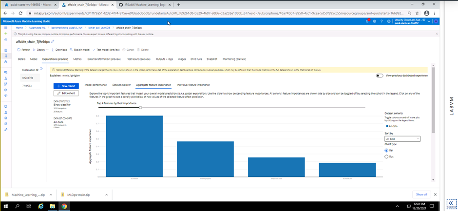
Screenshot 7: Explanation of the best model.
Screenshot 7 provides a preview on the explanation of the best model. The preview shows the top four features that will help predict the outcome from new data being fed to the model endpoint later in this project.
The third step in this project is to deploy the best model chosen from the Automated ML Experiment earlier.
In this step the configuration setup for the deployment of the best model is completed and the model is then deployed. A name was provided for the deployed model, a brief description, container type was set as an Azure Container Instance and authentication was enabled.
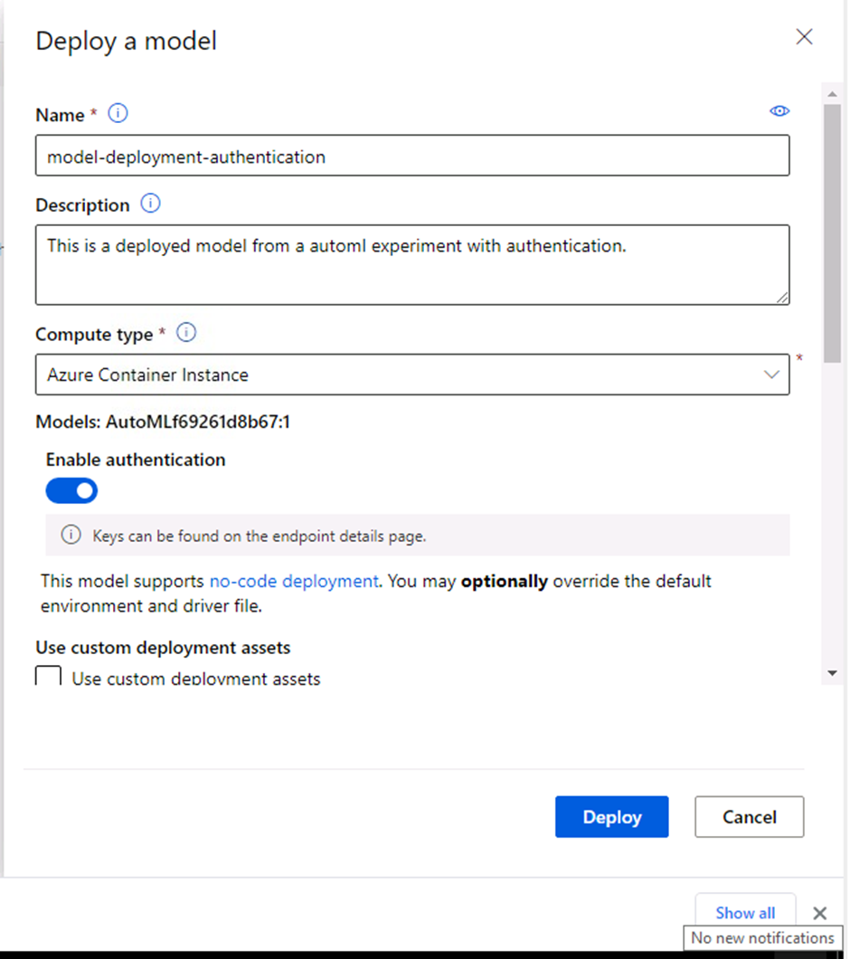
Screenshot 8: Model deployment setup.
Screenshot 8 shows the configuration information for the deployed model. The model name, description, compute type and authentication can be seen configured.
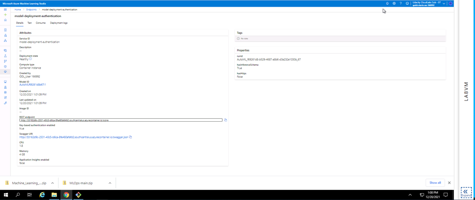
Screenshot 9: Deployed model details.
Screenshot 9 provides visual confirmation on the successful deployment of the best model. The deployment state can be seen as healthy. Information like the REST endpoint and Swagger URI is shown. These details will be used later in this project.
The fourth step in this project was to enable logging. In order to enable logging Azure Python SDK was used. The python file provided in the starter_files folder (logs.py) was inspected and in order to work correctly a config.json file needs to be downloaded. The config.json file contains detail about the Azure subscription and workspace. The logs.py file was then modified to include my deployed model name and a line added to enable Application Insights (service.update(enable_app_insights=True)). The logs.py file was executed in a terminal to enable Application Insights for the deployed model and to provide logging output.
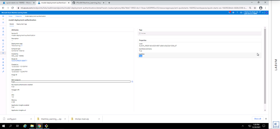
Screenshot 10: Application insights enabled.
Screenshot 10 is a visual confirmation that the Application Insights for the deployed model is enabled. This can be seen in the endpoints section under the details tab and scroling down to Application insights enabled.
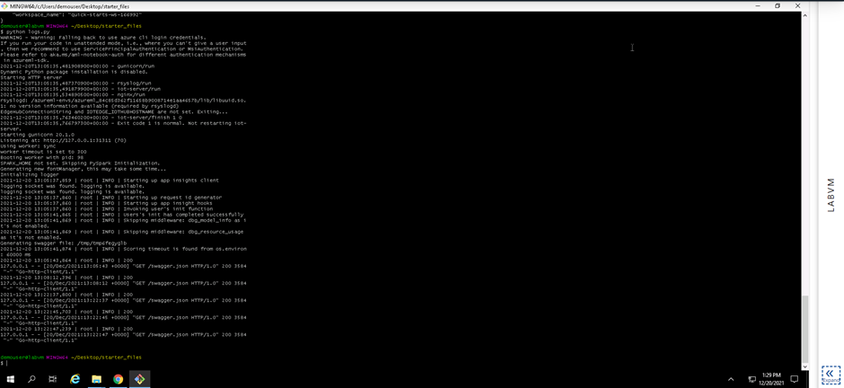
Screenshot 11: Execution of the logs.py file.
Screenshot 11 provides confirmation that the logs.py file was executed and provides logging output from the deployed model.
The fith step in this project was making use of Swagger Documentation to consume the deployed model endpoint. The following steps needs to be completed in order to consume the enpoint using Swagger:
- The swagger.json file for the deployed model was downloaded.
- The port number in the swagger.sh file was changed from 80 to 9000.
- Execute the swagger.sh file (This will download the latest Swagger container and will run on port 9000).
- Execute the serve.py file (This will start a Python server on port 8000).
- Open up a browser and go to localhost.
- Enter http://localhost:8000/swagger.json to interact with the Swagger instance running, showing the documentation for the HTTP API of the model.
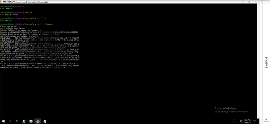
Screenshot 12: Execution of the swagger.sh file.
Screenshot 12 provides confirmation that the swagger.sh file was executed successfully. The execution of the swagger.sh file will download the latest Swagger container and will then run on port 9000.
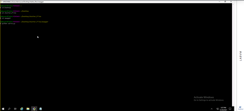
Screenshot 13: Execution of the serve.py file.
Screenshot 13 provides confirmation that the serve.py file was executed. This execution will start a local python server on port 8000.
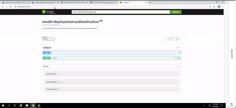
Screenshot 14: Swagger documentation running on a local host.
Screenshot 14 provides confirmation that a Swagger instance is running on a local host. The HTTP API methods and responses of the deployed model can be seen.
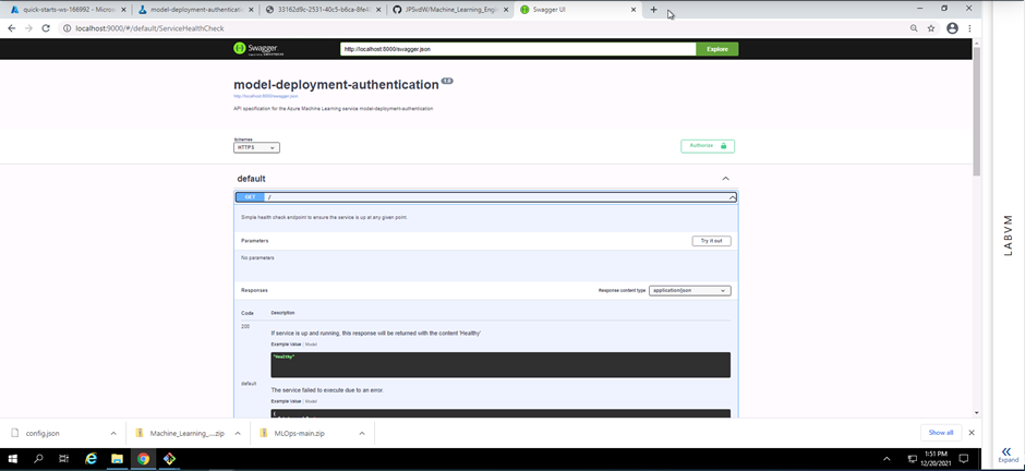
Screenshot 15: HTTP API GET method.
Screenshot 15 shows the details of the deployed model's HTTP API GET method. This is acomplished by expanding the GET field seen in screenshot 14.
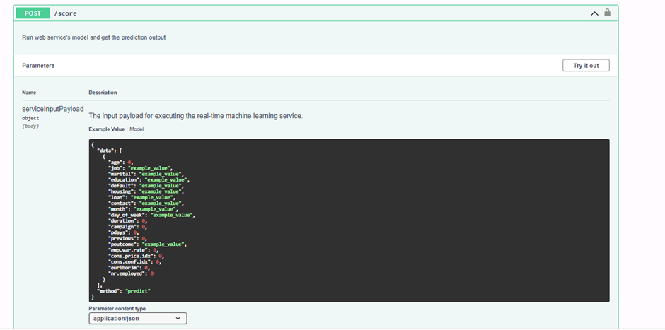
Screenshot 16: HTTP API POST method.
Screenshot 16 shows the details of the deployed model's HTTP API POST method. This is acomplished by expanding the POST field seen in screenshot 14. The data structure seen will be used to send requests to the model endpoint and to get a prediction response in a later step using the Python SDK.
The sixth step in this project was to consume the model endpoint using a python script.
The endpoints.py file was provided along with the starter_files folder. In order to interact with my deployed model, I had to make a few modifications to the endpoints.py file.
- Authentication was enabled for my deployed model and thus I had to fetch the scoring_uri and key from the consume tab of my deployed model in Microsoft Azure Machine Learning Studio and add it to the endpoints.py file.
- I added two sets of data to the endpoints.py file which will return two predictions on wheter these clients will make a deposit at the bank.
Screenshot 17: Execution of the endpoints.py file.
Screenshot 17 provides confirmation that the endpoints.py file was executed and two prediction responses was provided. The datastructure seen in screenshot 16 was added to the endpoint.py file with values for each field. When the endpoint.py file gets executed two data structures with values is sent to the model endpoint using the POST method and two prediction responses is delivered.
The seventh and final step in this project was to creat, publish and Consume a pipeline. The following screenshots shows that I created, published and consumed a pipeline.
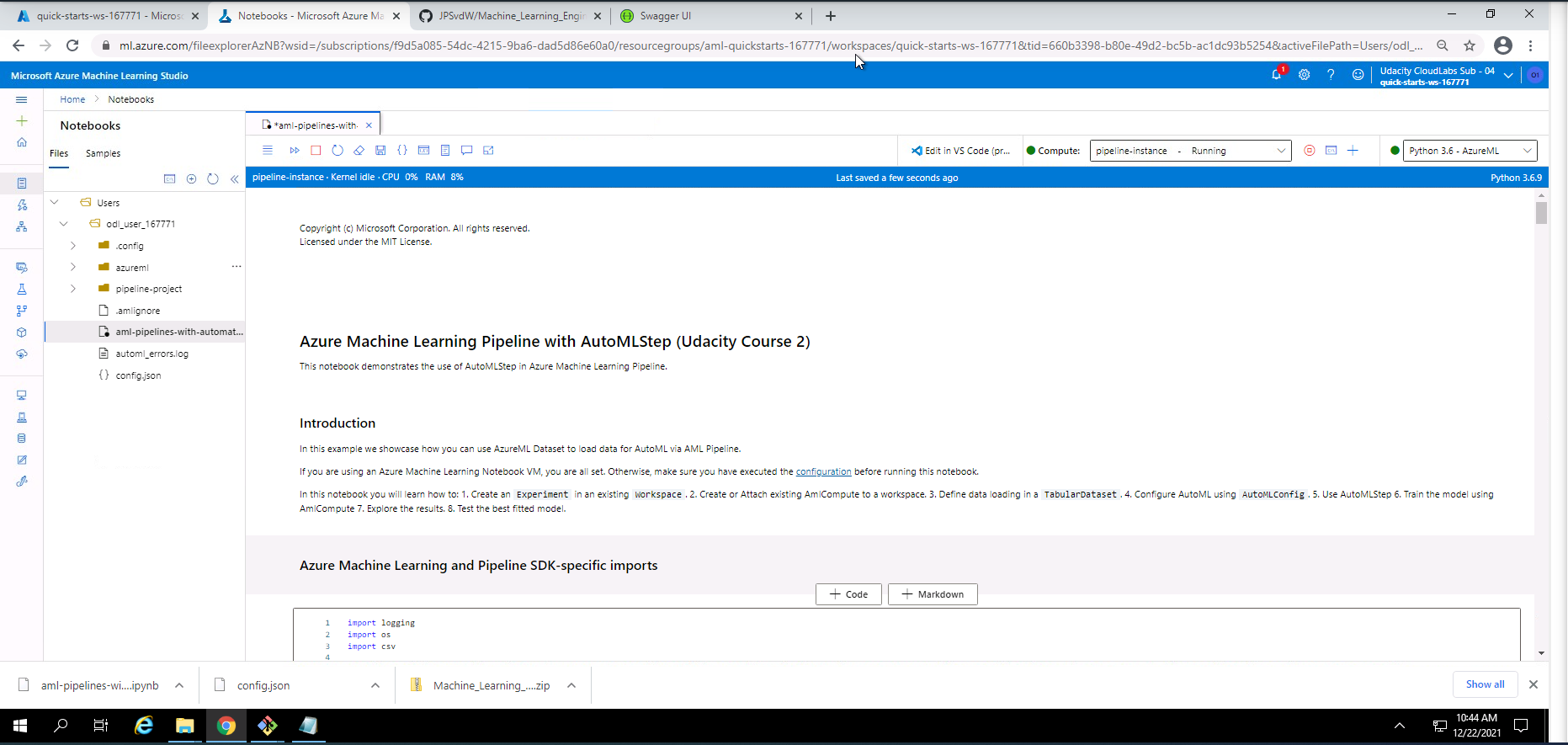
Screenshot 18: Using Jupyter Notebooks to create and publish a pipeline.
Screenshot 18 is a visual representation of the notebooks section in Microsoft Azure Machine Learning Studio where a file called aml-pipelines-with-automated-machine-learning-step.ipynb provided in the starter_files will be used to create and publish a pipeline.
The first step to run this Jupyter Notebooks file successfully is to upload the aml-pipelines-with-automated-machine-learning-step.ipynb file along with the config.json file to the notebooks section. The second step is to update all variables to match my workspace and environment. The third step is to run throug all the cells. The final step is to verify that the pipelines were created, were scheduled and are running.
The steps can be seen in the aml-pipelines-with-automated-machine-learning-step.ipynb file. I will briefly list the steps taken in this file:
1). Importing of Azure Machine learning and Pipeline SDK packages.
2). Initializing the workspace.
3). Creating an Azure ML Experiment.
4). Attaching or creating a new AMLCompute cluster.
5). Loading the dataset.
6). Viewing a small portion of the dataset.
7). Create an AutoML settings object.
8). Create Pipeline and AutoMLStep.
9). Examine the results.
10). Retrieve the best model.
11). Test the best model.
12). Publish the pipeline to the workspace and run the REST endpoint.
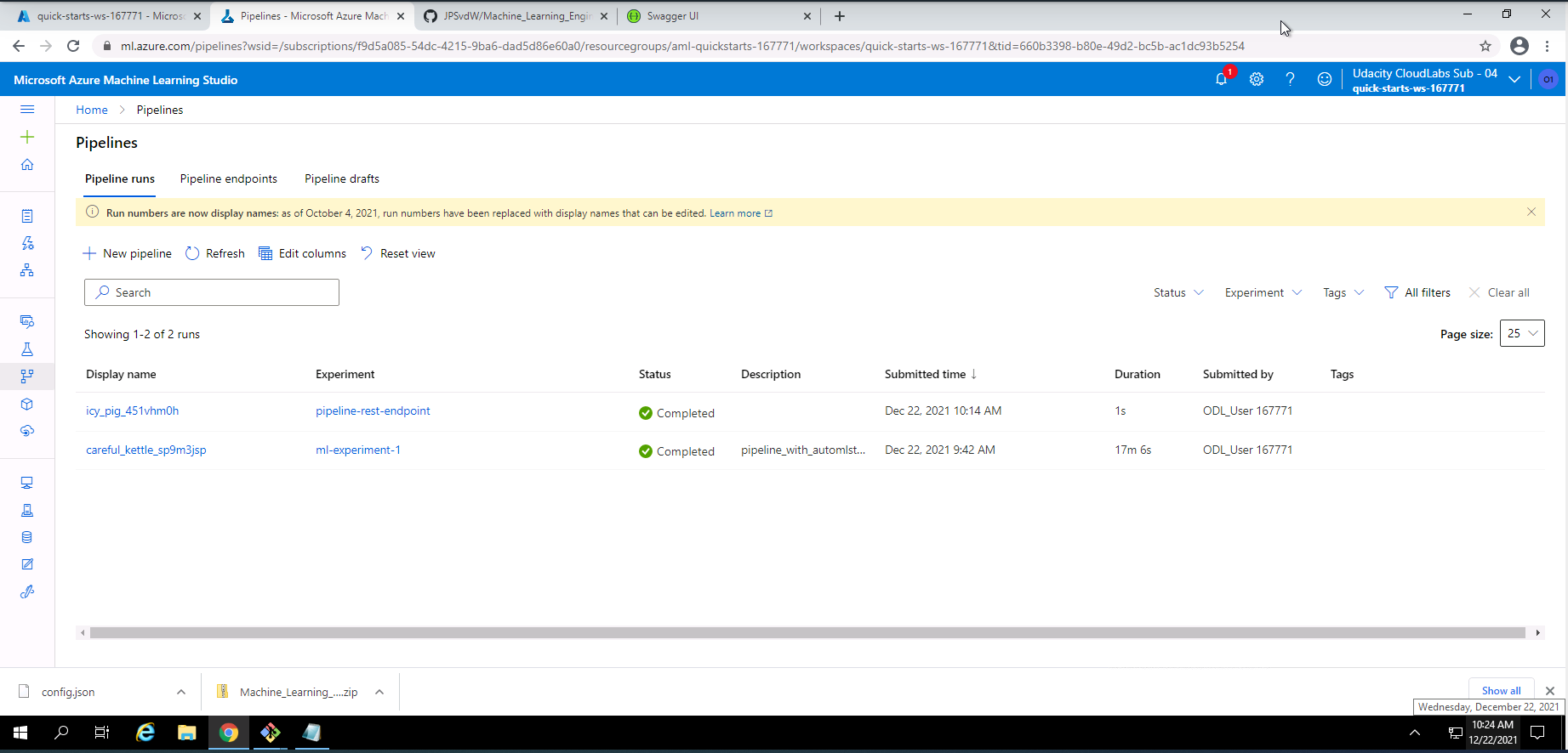
Screenshot 19: Pipeline runs successfully executed.
Screenshot 19 provides confirmation that the pipeline runs submitted from the Jupyter Notebook has been successfully completed. this information can be found under the piplines section under the pipeline runs tab.
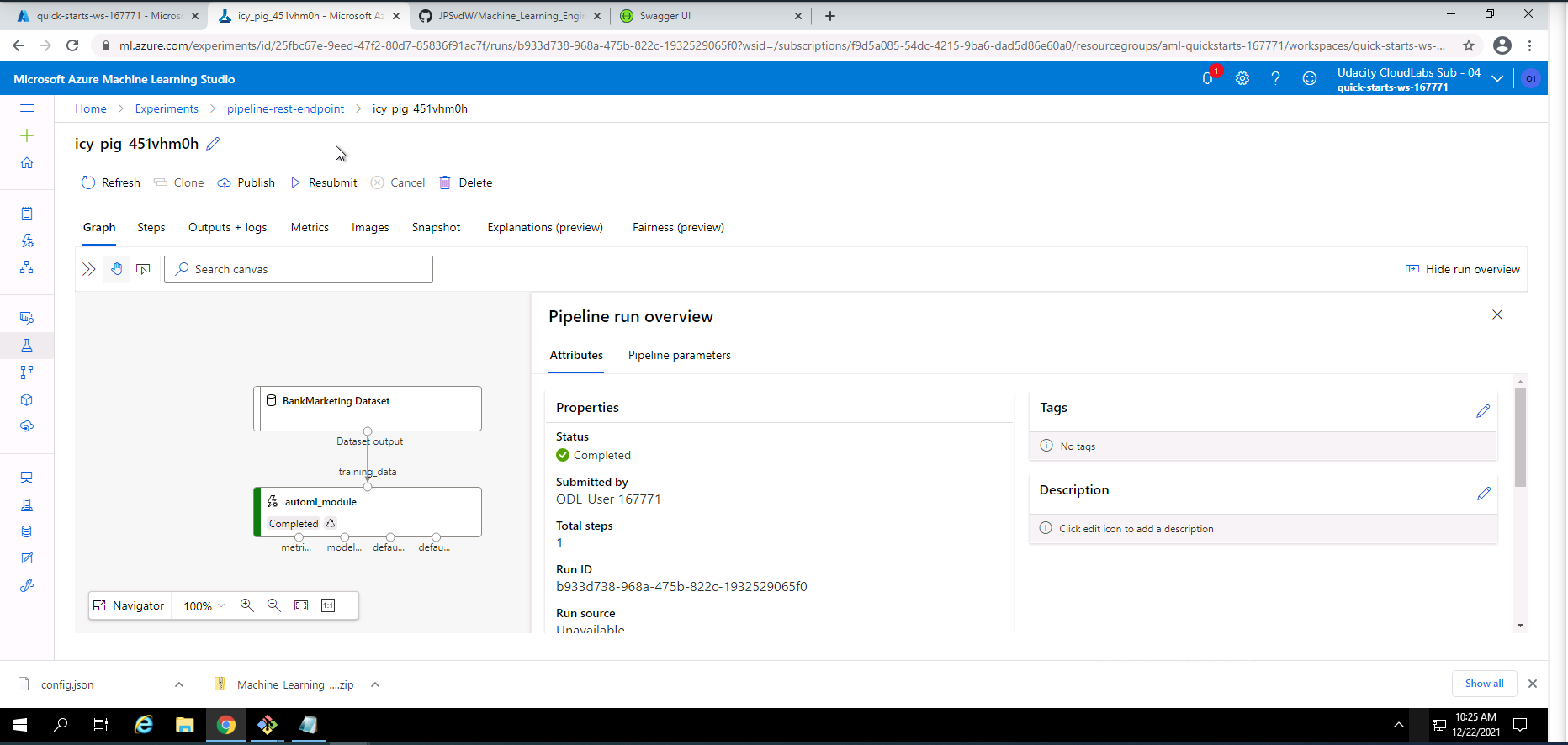
Screenshot 20: Pipeline REST endpoint run information.
Screenshot 20 shows some information regarding the pipeline REST endpoint run that was completed successfully. This screen can be found by clicking on the pipeline-rest-endpoint run link in screenshot 19.
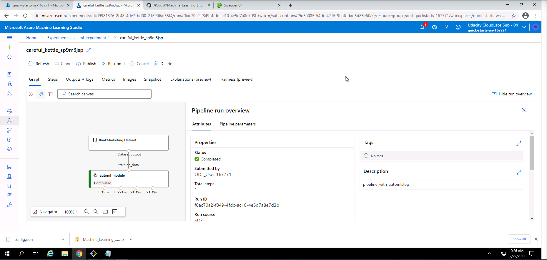
Screenshot 21: Pipeline experiment run information.
Screenshot 21 shows some information regarding the pipeline experiment run that was completed successfully. This screen can be found by clicking on ml-experiment-1 link in screenshot 19.
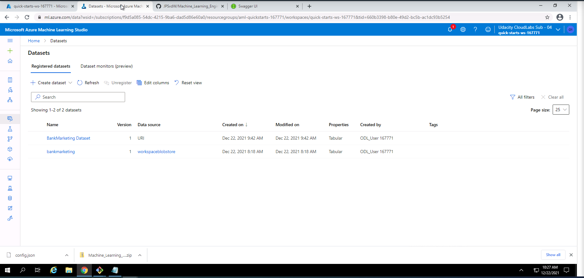
Screenshot 22: Registration of the bankmarketing dataset from the Jupyter Notebook.
Screenshot 22 confirms the registration of the bankmarketing dataset with the AutoML module initiated from the Jupyter Notebook. This screen can be found under the datasets section.

Screenshot 23: Pipeline REST endpoint experiment information.
Screenshot 23 provides information on the pipeline REST endpoint experiment. This screen can be accessed under the experiments section and selecting pipeline-rest-endpoint.
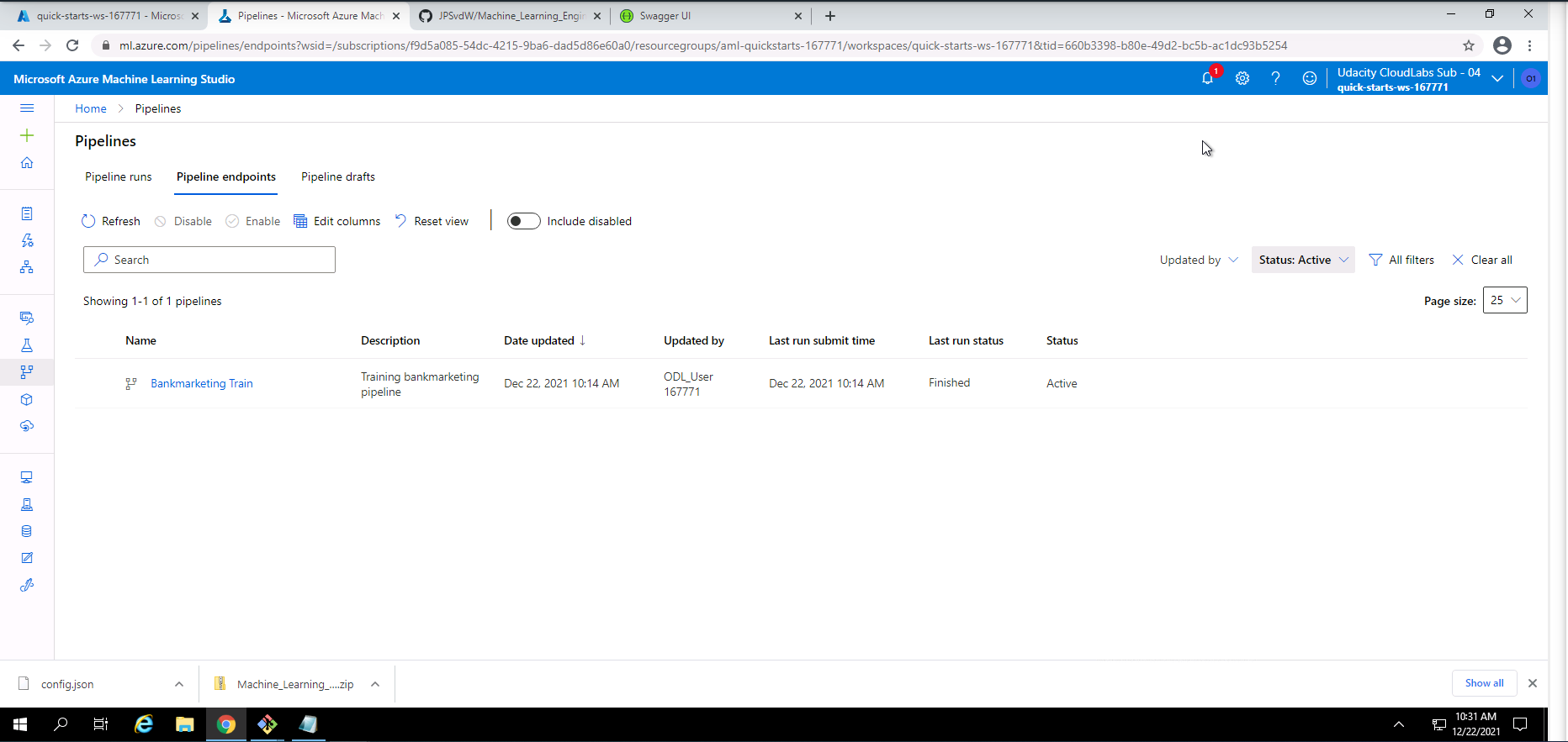
Screenshot 24: Confirmation that the pipeline REST endpoint is active.
Screenshot 24 provides confirmation that the pipeline REST endpoint is active. This screen can be found in the pipelines section under the pipeline endpoints tab.
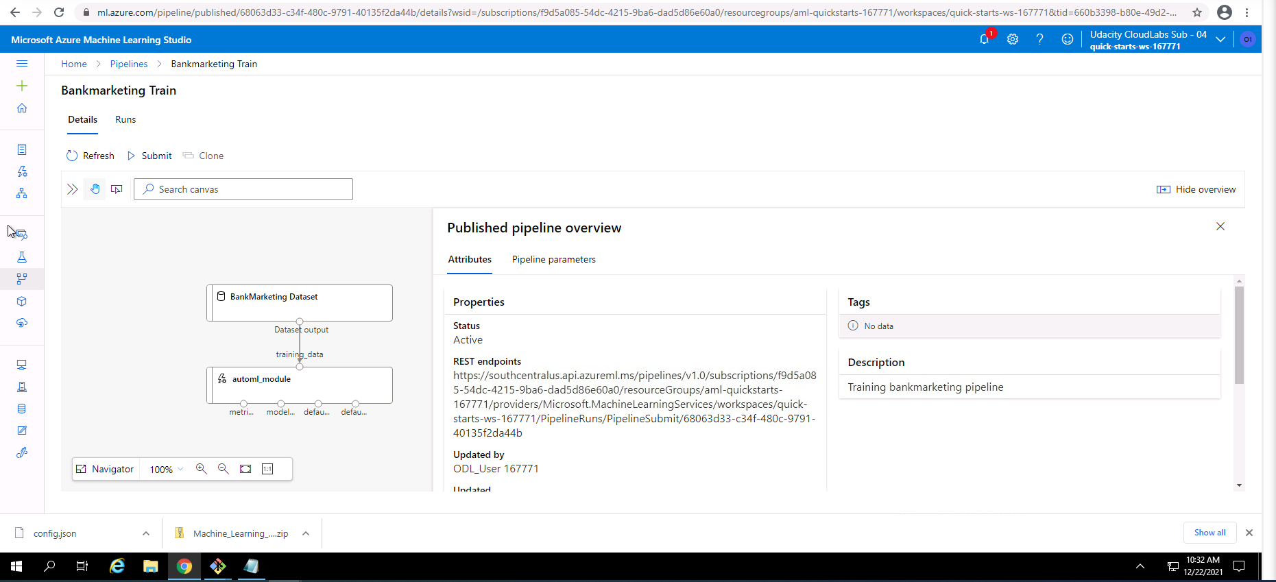
Screenshot 25: Published pipeline overview.
Screenshot 25 shows an overview of the Bankmarketing Train pipeline. This screen can be accessed from the pipelines section and clicking on the Bankmarketing Train link.
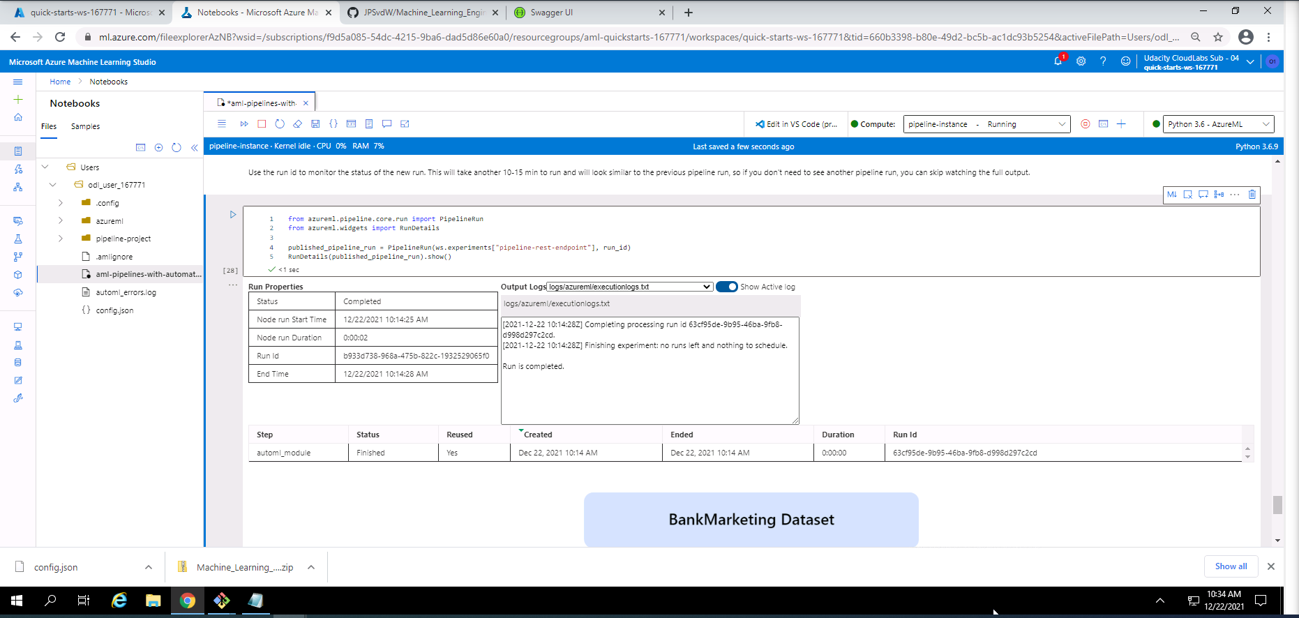
Screenshot 26: Use RunDetails Widget
Screenshot 26 shows the details regarding the pipeline runs within the "Use RunDetails Widget". This screen can be found under the Publish and run from REST endpoint section in the Jypyter Notebook.
The two screenshots below shows the scheduled run in ML studio.
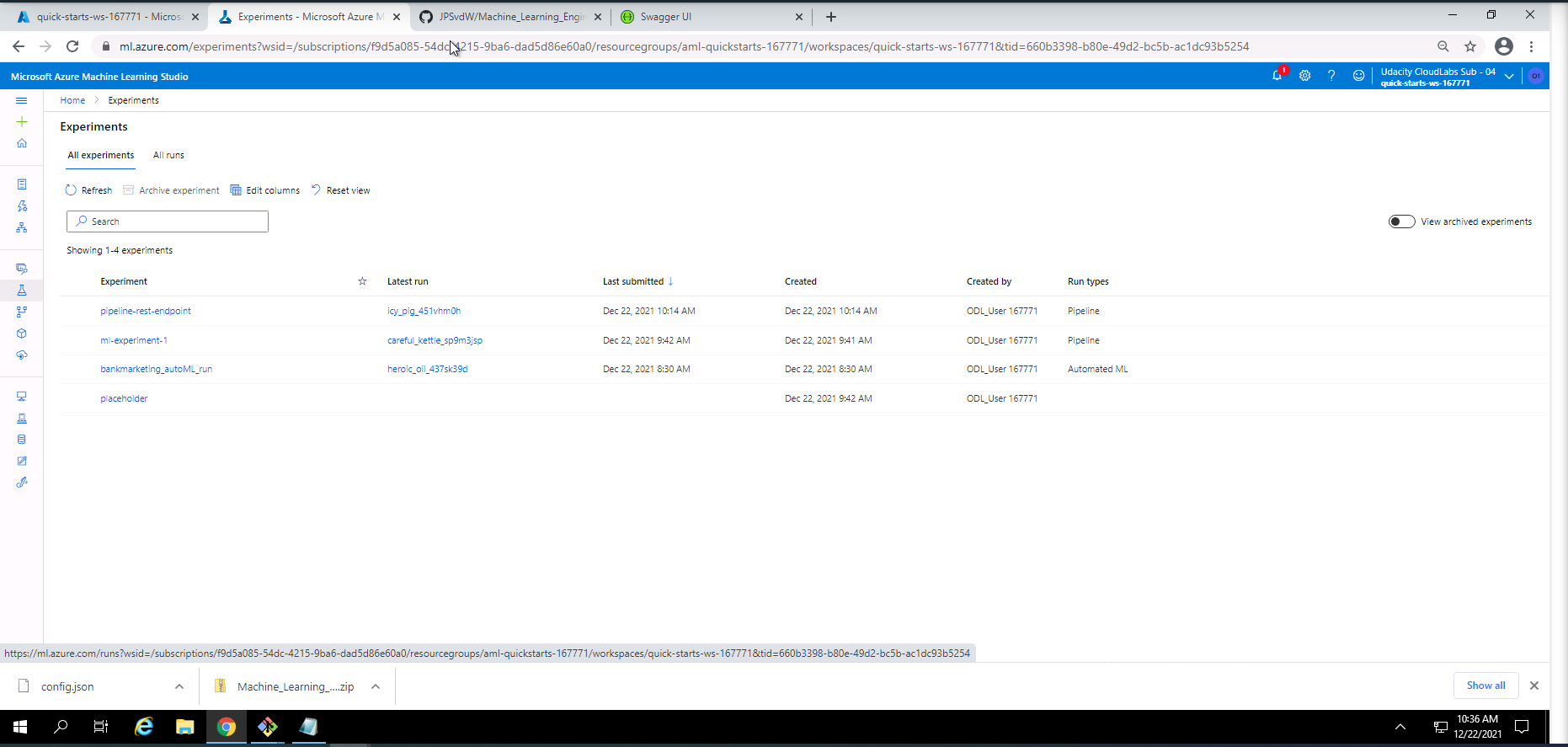
Screenshot 27: Scheduled runs in ML Studio.
Screenshot 27 lists the runs in Microsoft Azure Machine Learning Studio. This screen can be found under the experiments section ander the all experiments tab.
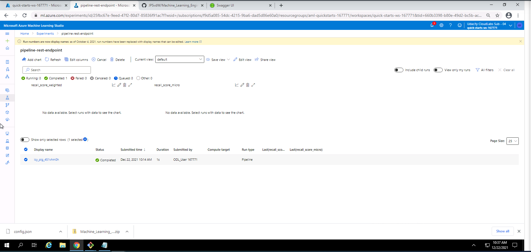
Screenshot 28: Pipeline REST endpoint experiment details.
Screenshot 28 shows the details regarding the pipeline REST endpoint experiment that was completed successfully. This screen can be found under the Experiments section and by clicking on pipeline-rest-endpoint.
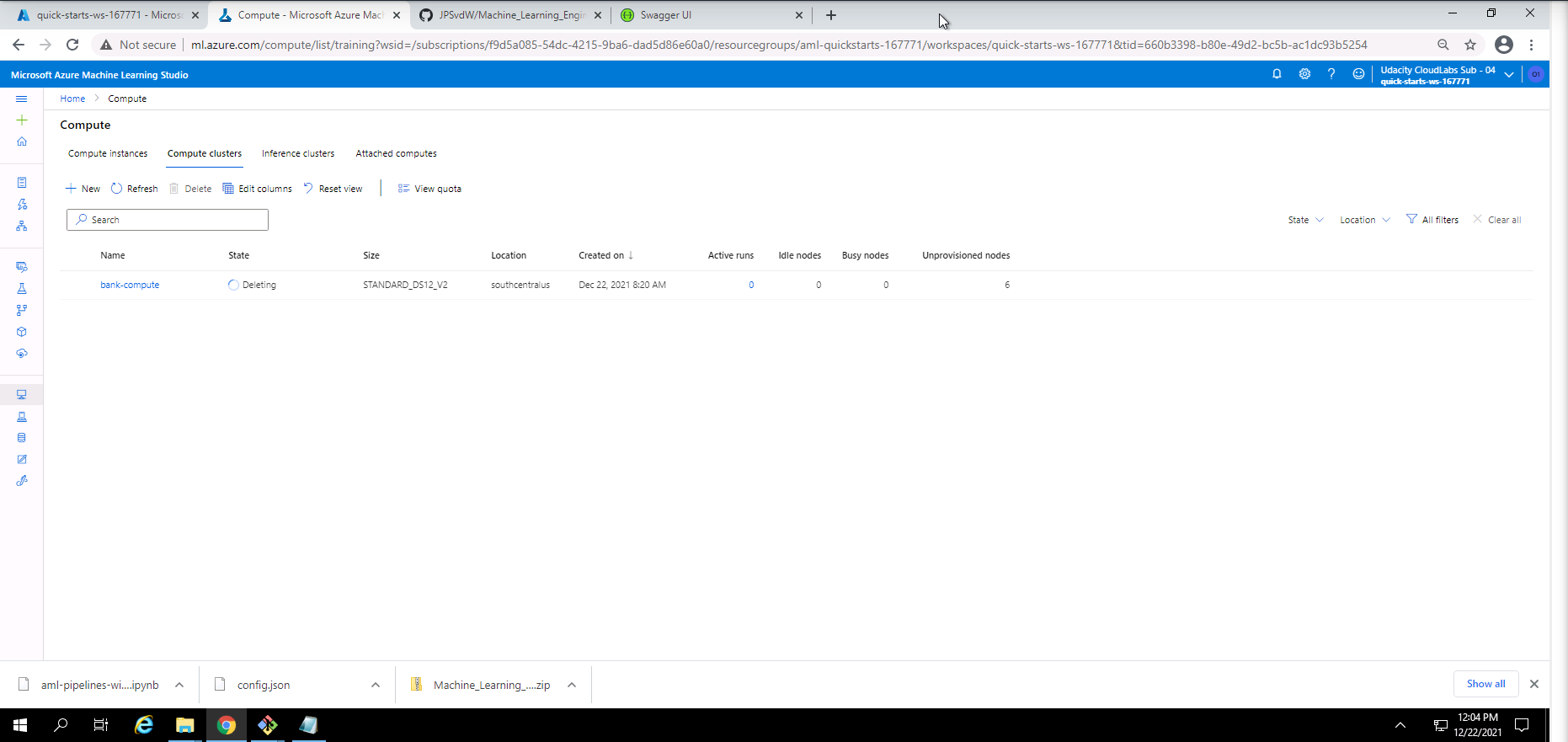
Screenshot 29: Compute cluster cleanup.
Screenshot 29 provides confirmation of the cleanup of the compute cluster used in this project. This was done by navigating to the compute section under the Compute clusters tab and deleting the active compute cluster.

Screenshot 30: Compute instance cleanup.
Screenshot 30 provides confirmation of the cleanup of the compute instance used in this project. This was done by navigating to the compute section under the Compute instances tab and deleting the active compute instance.
Screencast 1: Screencast demonstarating the steps taken during this project.
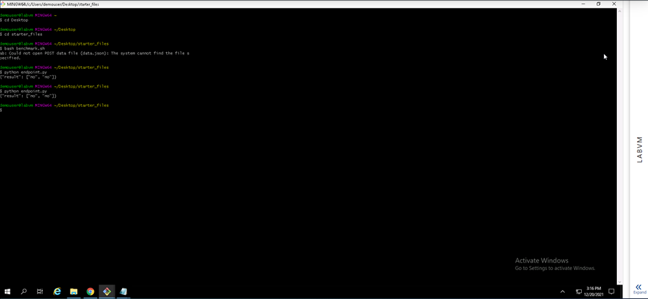
One of the standout suggestions was to run the Apache Benchmark (ab) against my deployed model's HTTP API. I had to make sure that the Apache Benchmark command-line tool is installed. Because the endpoint requires authentication, I had to replace the scoring_uri and key in the endpoint.py file with the correct uri and key that can be found under the consume tab of the deployed model. After executing the endpoint.py file, a data.json file will be generated. Only after the data.json file has been generated can the benchmark.sh file be executed. Before the benchmark.sh file can be executed the scoring_uri and key must be replaced. The benchmark.sh file was executed and a screenshot of the output is included below.
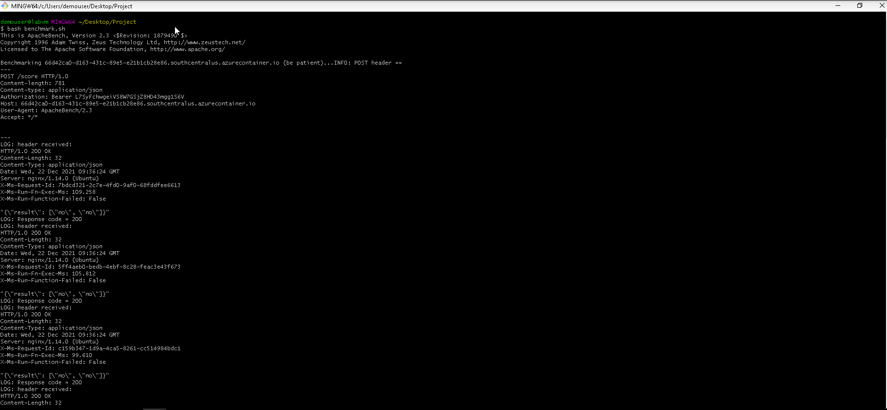
Screenshot 31: Execution and response from the Apache Bencmarking tool.
Screenshot 31 shows the successful execution and response of the Apache Benchmarking tool ran against my deployed model endpoint.
The output shows that the HTTP requests was executed successfully and also provides the prediction output from the model endpoint. Some more performace metrics like test time, number of successful requests, number of failed requests, total data transfered and received, metrics on connection times and percentage of requests served within a certain time was included in the response.
The full response is included as comments in the benchmark.sh file for further investigation.