This is a capstone project carried out by me to demonstrate my problem-solving skills in data analysis after completing the Google Data Analytics Professional Certification Course

I'm a junior data analyst recently hired by Cyclistic Company to work with the marketing analysis team. Cyclistic is a bike-share company in Chicago that feature more than 5800 bicycles and 600 dacking stations. Lily Morino is my manager and the director of marketing and he is responsible for the development of campaigns and initiative to promote the bike share program. My team is responsible for collecting,analyzing and reporting data that help guide Cyclistic marketing strategy. The approval of recommended marketing program is the task of the cyclistic executive team. Cyclistic has a flexible plan for the use of bikes,that the bike can be unlocked from one station and returned to any other station in the system any time. For the pricing: single_ride pass, full_day passes and are referred as casual_riders, riders who purchase an annual memberships and are referred as cyclistic_members. cyclistic finance analysts have concluded that annual_memberships are much more profitable than casual_riders. The Director of marketing believes that the future of the company success depends on maximizing the number of annual memberships and that will be the key to future growth too and there's a very good chance to convert casual_riders to cyclistic_members. Consequently, Morino set a clear goal which is to design marketing strategies aimed at converting casual_riders to cyclistic_members. By now my team wants to understand how casual riders and annual members use cyclistic bikes differently, from these insights the marketing team will design a new marketing strategy to convert casual riders to annual members.
Morino and the team are interested in analyzing the historical bikers trip data to identify trends. This future marketing program is guided by three questions:
1- how do annual members and casual riders use cyclistic bikes differently?
2- why would casual riders buy cyclistic annual membership?
3- how can cyclistic use digital media to influence casual riders to become members?
Morino has assigned me the first question, and this task is an opportunity for me as a junior data analyst to show my skills in the domain by applying my knowledge in this field of data analysis by following the different phases : ask, prepare, process, analyze, share and act. The goal of the team is clear that is to have a successful marketing campaign toward the casual riders, in that we need to understand how the two types of riders behave differently? now that the asked question is clear: how do annual members and casual riders use Cyclistic bikes differently? all my job is to focus on this question in the aim to enhance the mission of my team by responding to the stakeholders expectations, enabling them to take a data driven decisions.
The instruction of my manager is to use the historical data of the last twelve months collected by the company and kept herelink. and he gave me a week to finish this task.
I prepared a new folder in my pc called "bike_trips" to download the needed data.They are twelve files in zip format. The files are unzipped and each file is an csv file for one month period starting from August 2021 to July 2022. this data was provided by the and it's relevent, complete, comprehensive, current and cited.
R studio was used as a suitable tool for this task, it can enables me to perform different tasks such as importing the data,wrangling it, analyzing it, visualising it, documenting and sharing results by markdown files. To start with, data was imported to R studio after selecting appropriate directory the unzipped and downloaded CSV files was located on the computer. After which, necessary packages was installed and loaded into R Studio.
library(tidyverse) library(lubridate)
August_2021_tripdata <- read_csv("Aug_2021.csv") September_2021_tripdata <- read_csv("Sept_2021.csv") October_2021_tripdata <- read_csv("Oct_2021.csv") November_2021_tripdata <- read_csv("Nov_2021.csv") December_2021_tripdata <- read_csv("Dec_2021.csv") January_2022_tripdata <- read_csv("Jan_2022.csv") February_2022_tripdata <- read_csv("Feb_2022.csv") March_2022_tripdata <- read_csv("Mar_2022.csv") April_2022_tripdata <- read_csv("Apr_2022.csv") May_2022_tripdata <- read_csv("May_2022.csv") June_2022_tripdata <- read_csv("June_2022.csv") July_2022_tripdata <- read_csv("July_2022.csv")
str(August_2021_tripdata) str(September_2021_tripdata) str(October_2021_tripdata) str(November_2021_tripdata) str(December_2021_tripdata) str(January_2022_tripdata) str(February_2022_tripdata) str(March_2022_tripdata) str(April_2022_tripdata) str(May_2022_tripdata) str(June_2022_tripdata) str(July_2022_tripdata)
colnames(August_2021_tripdata) colnames(September_2021_tripdata) colnames(October_2021_tripdata) colnames(November_2021_tripdata) colnames(December_2021_tripdata) colnames(January_2022_tripdata) colnames(February_2022_tripdata) colnames(March_2022_tripdata) colnames(April_2022_tripdata) colnames(May_2022_tripdata) colnames(June_2022_tripdata) colnames(July_2022_tripdata)
It clearly shows that column are consistent with no errors, now we can bind our data together for easy analysis.
bike_trips<-rbind(August_2021_tripdata,September_2021_tripdata,October_2021_tripdata,November_2021_tripdata,December_2021_tripdata,January_2022_tripdata,February_2022_tripdata,March_2022_tripdata,April_2022_tripdata,May_2022_tripdata,June_2022_tripdata,July_2022_tripdata)
glimpse(bike_trips)
bike_trip<- bike_trips[!duplicated( bike_trips), ]
bike_trips$ride_period <- difftime(bike_trips$ended_at, bike_trips$started_at, units = "mins")
bike_trips$ride_period %>% head(10)
Convert 'started_at' column from character to POSIXct to extract hour,day,month from date
bike_trips$started_at<-as.POSIXct(bike_trips$started_at)
bike_trips$start_hour<-format(bike_trips$started_at, "%H") bike_trips$day<- format(bike_trips$started_at, "%a") bike_trips$month<- format(bike_trips$started_at, "%b")
After exploring the ride_period values, we conclude that it is essential to remove the outliers with the aim to have meaningful values in our analysis(outliers= <1st qu. 1.5 & >3rd qu 1.5)
bike_trips[!(bike_trips$ride_period < 6.37 *1.5 | bike_trips$ride_period> 20.60 *1.5), ]
bike_trips$ride_period <- as.numeric(as.character(bike_trips$ride_period)) is.numeric(bike_trips$ride_period)
average on days of the week
bike_trips$avg_daily_ride<-aggregate(bike_trips$ride_period ~ bike_trips$member_casual + bike_trips$day , FUN=mean)
Average monthly ride
average_monthly_ride<-aggregate(bike_trips$ride_period ~ bike_trips$member_casual +bike_trips$month, FUN = mean)
Average hourly ride
average_hourly_ride<-aggregate(bike_trips$ride_period ~ bike_trips$member_casual + bike_trips$start_hour, FUN = mean)
Average ride by bike type
average_ride_type<-aggregate(bike_trips$ride_period ~ bike_trips$member_casual + bike_trips$rideable_type, FUN = mean)
riders distribution
table(bike_trips$member_casual)
by days of the week
daily_ride_trip<-bike_trips %>% group_by(member_casual, day) %>% summarise(number_of_rides = n(), .groups = 'drop') %>% arrange(day)
by hour
hourly_ride_trip<-bike_trips %>% group_by(member_casual, start_hour) %>% summarise(number_of_rides = n(), .groups = 'drop') %>% arrange(start_hour)
by month
bike_trips %>% group_by(member_casual, month) %>% summarise(number_of_rides = n(), .groups = 'drop') %>% arrange(month)
ride_no_member<-bike_trips%>% group_by(rideable_type, member_casual) %>% summarize(number_of_rides = n(), .groups = 'drop')
Top members stations *Create data frame containing only members riders
member_trips <- bike_trips[bike_trips$member_casual == 'member',]
top_5_start_stations_members
top5_member_start_stations<-member_trips %>%drop_na(start_station_name) %>% group_by(start_station_name, member_casual,start_lat, start_lng)%>% summarise(station_count = n(), .groups='drop')%>% arrange(desc(station_count)) %>%head(n=5)
top_5_end_station_members
top5_member_end_stations<-member_trips %>%drop_na(end_station_name) %>% group_by(end_station_name, member_casual,end_lat, end_lng)%>% summarise(station_count = n(), .groups='drop')%>% arrange(desc(station_count)) %>%head(n=5) top5_member_end_stations
Top casuals stations *Create data frame containing only casuals riders
casual_trips <- bike_trips[bike_trips$member_casual == 'casual',]
top_5_casual_start_stations
top5_casual_start_stations<-casual_trips %>%drop_na(start_station_name) %>% group_by(start_station_name, member_casual,start_lat, start_lng)%>% summarise(station_count = n(), .groups='drop')%>% arrange(desc(station_count)) %>%head(n=5)
top_5_casual_end_stations
top5_casual_end_stations<-casual_trips %>%drop_na(end_station_name) %>% group_by(end_station_name, member_casual,end_lat, end_lng)%>% summarise(station_count = n(), .groups='drop')%>% arrange(desc(station_count)) %>%head(n=5)
top_start_stations<-rbind(top5_member_start_stations, top5_casual_start_stations)
top_end_stations <-rbind(top5_member_end_stations, top5_casual_end_stations)
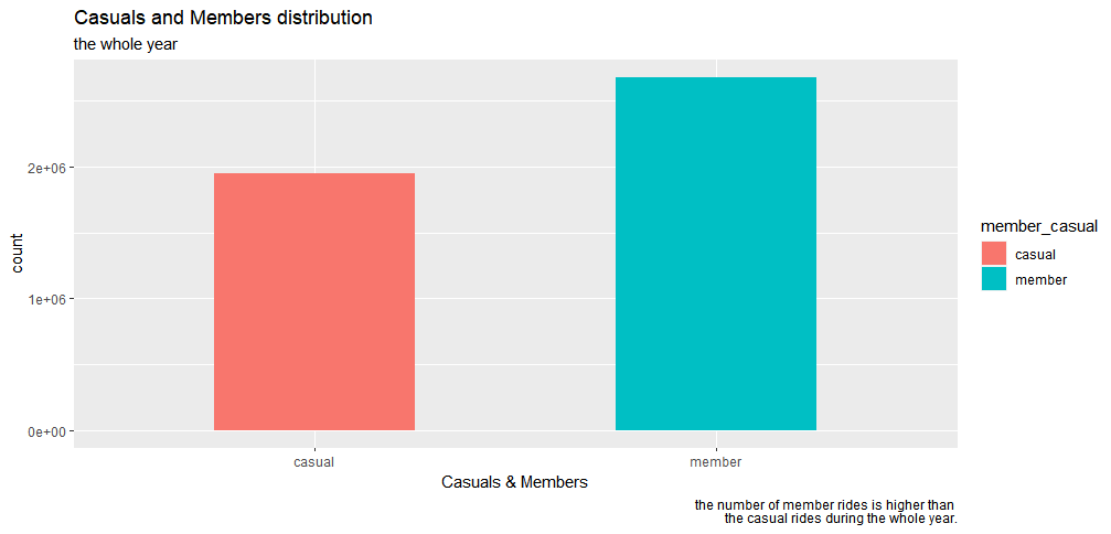
year_member_casual_distribution<-ggplot(bike_trips, aes(member_casual, fill=member_casual)) +geom_bar(width=0.5) + labs(x="Casuals & Members", title="Casuals and Members distribution", subtitle="the whole year ", captions=" the number of member rides is higher than the casual rides during the whole year.")
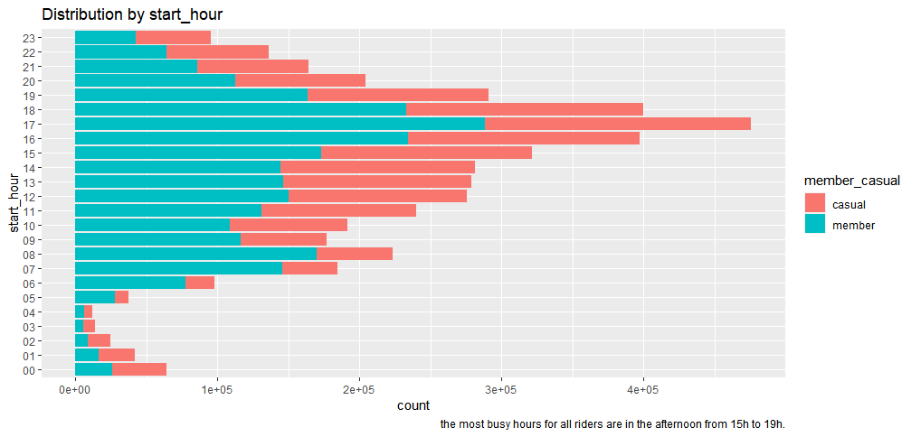
member_casual_hour<-bike_trips %>%ggplot(aes(start_hour, fill=member_casual))+geom_bar() member_casual_hour+labs(x="start_hour", title="Distribution by start_hour", caption = " the most busy hours for all riders are in the afternoon from 15h to 19h.") + coord_flip()
make the week days in order
bike_trips$day<- ordered(bike_trips$day, levels = c("Mon", "Tue", "Wed","Thu", "Fri", "Sat", "Sun"))
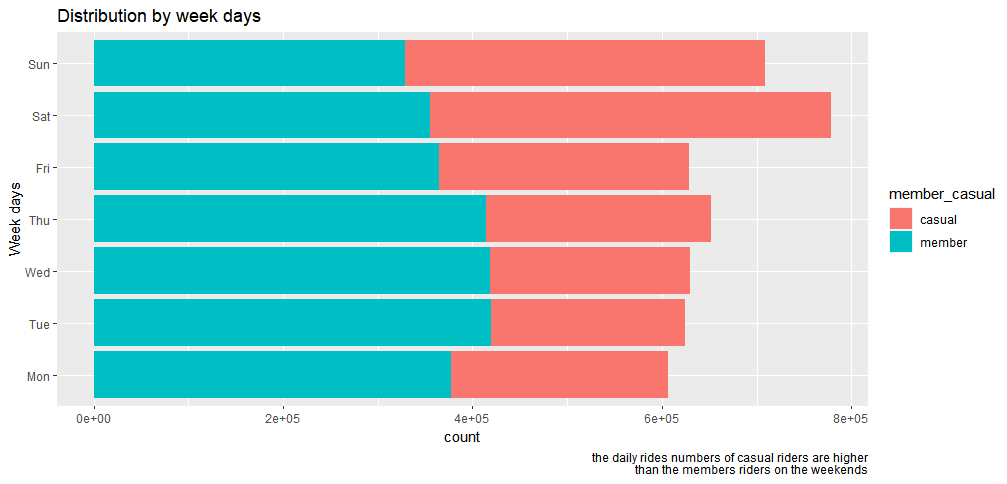
member_casual_day<-ggplot(bike_trips, aes(day, fill=member_casual))+ geom_bar()+coord_flip() member_casual_day+labs(x="Week days", title="Distribution by week days", captions = "the daily rides numbers of casual riders are higher than the members riders on the weekends")
order the month
bike_trips$month<- ordered(bike_trips$month, levels = c("Jan", "Feb", "Mar","Apr", "May", "Jun", "Jul","Aug", "Sep", "Oct","Nov", "Dec"))
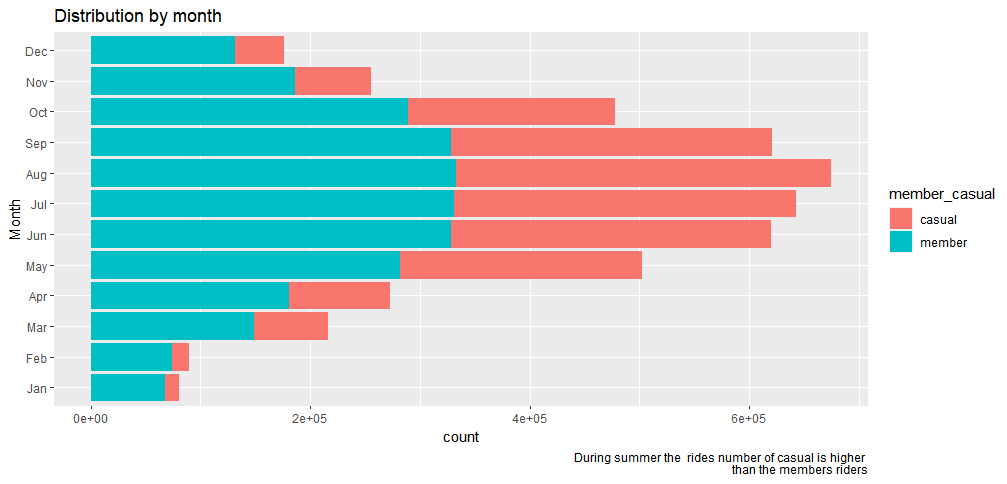
bike_trips %>% ggplot(aes(month, fill=member_casual)) + geom_bar() + labs(x="Month", title="Distribution by month", caption=" in the festival period the rides number of casual is higher than the members riders") + coord_flip()
ride_duration_month<-bike_trips %>% group_by(member_casual, month,rideable_type ) %>% summarise(average_ride_period=mean(ride_period) ,.groups = 'drop') %>% arrange(rideable_type)
ride_duration_month%>% ggplot(aes(month,as.numeric(average_ride_period), colour= member_casual))+geom_point()+ facet_wrap('rideable_type') + theme(axis.text.x = element_text(angle = 90))+ labs(title="Monthly average rides durations by bikes type", caption = " the highest average is by casual riding docked bikes ")

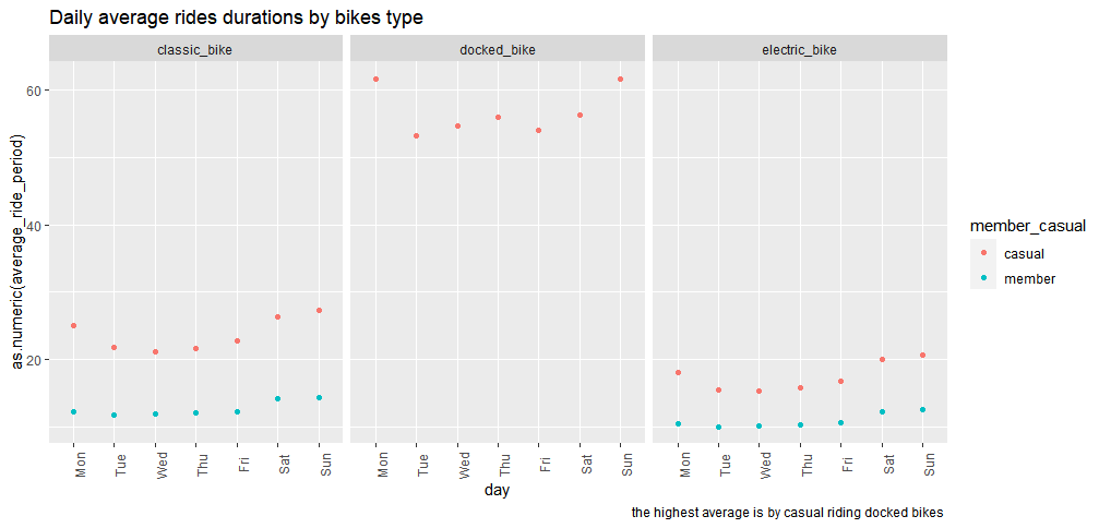
ride_duration_day<-bike_trips %>% group_by(member_casual, day,rideable_type ) %>% summarise(average_ride_period=mean(ride_period),.groups = 'drop') %>% arrange(rideable_type)
ride_duration_day%>% ggplot(aes(day,as.numeric(average_ride_period), colour= member_casual))+ geom_point()+facet_wrap('rideable_type') + theme(axis.text.x = element_text(angle = 90))+ labs(title="Daily average rides durations by bikes type", caption = " the highest average is by casual riding docked bikes ")
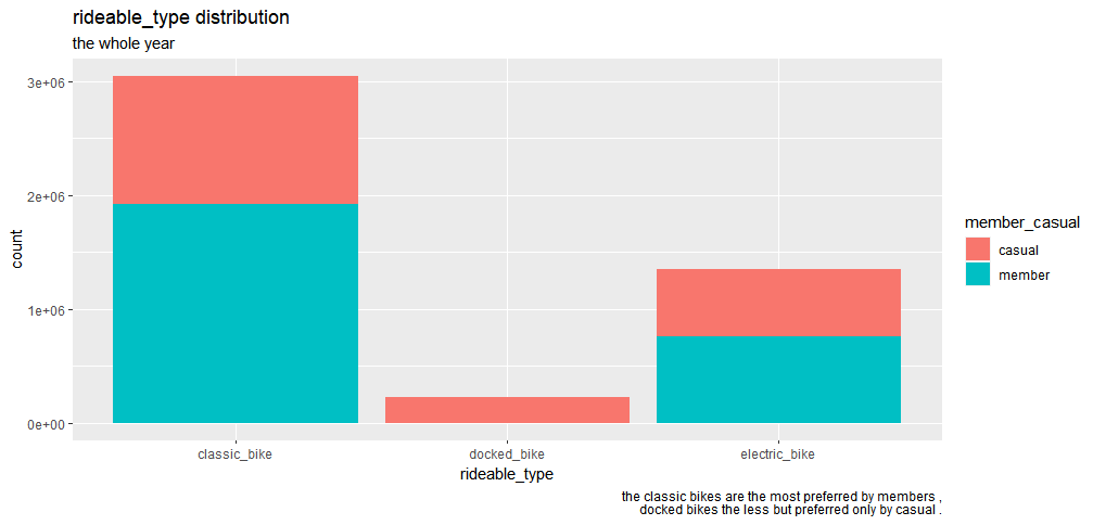
type<-ggplot(bike_trips, aes(rideable_type, fill=member_casual)) + geom_bar() type+ labs(x="rideable_type", title="rideable_type distribution",subtitle="the whole year ", captions=" the classic bikes are the most preferred by members , docked bikes the less but preferred only by casual .")
- The cyclystic bike company should create a digital application "cyclistic ride" highlighting the benefits of annual membership and encourage all riders to use it.
- Improve Chicago social media preence to introduce the benefits of annual memberships.
- Organise bicycle ride competitions for customers every summer period. This lures other passionate bicylcle riders to enlist our services and thus be members.