---

PAGEpy - Predictive Analysis of Gene Expression with Python

Overview

PAGEpy (Predictive Analysis of Gene Expression in Python) is a Python package designed to easily test if a multi-layered neural network could produce a reasonable estimate of a target variable given a gene expression data set. This package is compatible with both single-cell and bulk RNA sequencing datasets. It requires four input files placed in a single directory:

1. A counts matrix, where genes are rows and cells or samples are columns (.mtx).
2. A text file containing the list of all gene names (.txt).
3. A text file containing the list of all sample/barcode names (.txt.).
4. A CSV file with the target variable of interest (.csv).

This repository provides code to format these datasets, split them into training and test groups, and select highly variable genes (HVGs) to be used as features for a neural network. The network is trained using a custom protocol aimed at minimizing overfitting and training set memorization.

Several customization options are available for different aspects of the process. The repository also includes a Particle Swarm Optimization (PSO) pipeline designed to refine the feature set. This pipeline generates multiple randomized subsets of the initial set of HVGs and iteratively optimizes them using PSO.

To evaluate each feature set, neural networks are trained for a small number of epochs, with performance assessed through repeated trials and averaging to ensure reliable estimates. Additionally, each feature set is tested across multiple K-folds within the training dataset. A variety of parameters are available for tuning and customization at every stage of this process.

The end result of the PSO pipeline is a set of features, based solely on the training dataset, that could potentially improve the model’s generalizability.

The codebase also includes various plotting scripts for evaluating the model's performance.

Table of Contents

• Installation
• Usage
• Project Organization
• Function and class descriptions
• Contributing
• License
• Contact

Installation

pip install PAGEpy

Usage

To get started, first open your script or notebook and import the necessary packages:

from PAGEpy import PAGEpy_plot
from PAGEpy import pso
from PAGEpy.format_data_class import FormatData
from PAGEpy.pred_ann_model import PredAnnModel
import pickle
import pandas as pd
from PAGEpy import PAGEpy_utils

PAGEpy_utils.init_cuda()

This ensures that all required packages are imported and enables GPU memory growth.

Formatting the Data

Next, you need to format your data so it can be passed to the relevant classes and functions within the PAGEpy codebase.

current_data = FormatData(data_dir = '/home/your_data_dir/',
        test_set_size=0.2,
        random_seed=1,
        hvg_count = 1000)

This instantiates the FormatData class, which requires a directory containing the following four files:

1. A counts matrix (.mtx), where genes are rows and cells/samples are columns.
2. A text file containing the list of all gene names.
3. A text file containing the list of all sample/barcode names.
4. A CSV file with the target variable of interest.

If you're working with a sparse matrix of class dgCMatrix in R, you can easily produce the required file types either in R or using an R API within Python.

library(Matrix)

counts <- readRDS('sparse.RNA.counts.rds')
writeMM(counts, "sparse.RNA.counts.mtx")

write.table(rownames(counts), "genes.txt", quote=FALSE, row.names=FALSE, col.names=FALSE)
write.table(colnames(counts), "barcodes.txt", quote=FALSE, row.names=FALSE, col.names=FALSE)

The FormatData class will automatically generate a list of genes for training the model, which is saved in the local directory as hvgs.pkl. This gene list is also available within the FormatData object. It’s preferred to load it from the file like this:

genes_path = '/home/your_path/hvgs.pkl'

with open(genes_path, 'rb') as f:
    current_genes = pickle.load(f)

Training the Model

Now, you can pass the genes list and FormatData object to the PredAnnModel class.

current_model = PredAnnModel(current_data,current_genes,num_epochs=500,auc_threshold=1)

The model offers many customization options, but only the input data, feature list, and number of epochs are required arguments. For a complete list of optional input arguments, refer to the class docstring (e.g., help(PredAnnModel)) or read the descriptions below in this README. Many of these options are related to regularization techniques.

Several features make this model effective:

1. The learning rate can be adjusted dynamically based on performance metrics during training.
2. A percentage of the training data is hidden during each epoch to reduce overfitting and prevent training data set memorization.
3. Target variable balancing is applied during the mini-batch training process.
4. The input layer of the classifier automatically scales based on the number of features passed to the model.

Once the class is instantiated, the model provides an update on the training progress every 10 epochs. For example, here is the output after epoch 40:

Epoch 40, Avg Outcome Loss: 0.2897, Train AUC: 0.9569, Train Accuracy: 0.8883, Test AUC: 0.9188, Test Accuracy: 0.8528

Evaluating the Model

After training the model, you can view its progress and metrics by running:

PAGEpy_plot.evaluate_model(current_model, current_data)

This will output:

max train accuracy: 1.0
max train auc: 1.0
max test accuracy: 0.87
max test auc: 0.93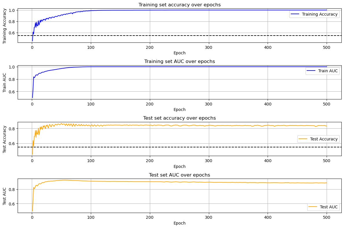

In this case, the model is predicting whether a cell is infected with HIV, using only the endogenous transcriptome.

Feature Set Optimization

If you're not entirely satisfied with the model's performance, you can adjust various parameters and increase the number of epochs. You can also expand or narrow the feature set. Alternatively, you can use the Particle Swarm Optimization (PSO) algorithm included in PAGEpy to optimize the feature set.

You can execute the PSO algorithm as follows:

best_solution, best_fitness = pso.binary_pso(current_genes, current_data, 200, 15,  C1 = 2, C2 = 1.5)

The binary_pso function uses the training data set generated by the FormatData class. With the pre-selected gene set, it randomly selects features for a specified number of population members (in this case, n=200) or particles. It then trains models for each feature set or particle. The model architecture used for evaluating each particle is similar to PredAnnModel, but with a simpler training regimen and fewer regularization elements. The models are trained for 50 epochs.

The PSO function works as follows:

After initializing a random set of particles, each particle is assigned a random velocity. The fitness of each particle is then evaluated by training across 5 K-folds (derived from the training data) and the final Test AUC is averaged across folds, this evaluation is calculated multiple times (user-specified) for each particle due to the semi-stochastic nature of the model training. Then velocity of each particle is updated as such:

$$ v_i^{(t+1)} = w v_i^{(t)} + c_1 r_1 (pbest_i - x_i^{(t)}) + c_2 r_2 (gbest - x_i^{(t)}) $$

where:

• w is the inertia weight (controls how much the previous velocity is retained).
• c1 and c2 are the acceleration coefficients (control the influence of pbest and gbest). Higher c1 values will lead to greater exploration whereas higher c2 values will lead to more exploitation and earlier convergence.
• r1 and r2 are random number values between 0 and 1.
• $x_i^{(t)}$ is the current position of particle 𝑖.

The position of each particle is then updated using:

$$ x_i^{(t+1)} = x_i^{(t)} + v_i^{(t+1)} $$

This produces a new particle vector which is then passed through a sigmoid function and allows each particle to be updated in response to past personal and group performance. In each iteration, each particle will update its personal best or pbest if the new position is better. The global gbest is updated if any particle achieves a better solution than the current gbest.

These steps are then repeated for a number of user-specified iterations. If the algorithm works well, there should be an improvement in the average and maximum test AUC values.

Since this algorithm can take a long time to run, it’s helpful to monitor its progress. The binary_pso function will produce two local files that you can load and use to track progress:

pso_df = pd.read_pickle("pso_fitness_scores.pkl")
pso_dict = pd.read_pickle("pso_particle_history.pkl")

PAGEpy_plot.plot_pso_row_averages(pso_df)
PAGEpy_plot.plot_hamming_distance(pso_dict)
PAGEpy_plot.plot_sorted_frequencies(pso_dict, pso_df)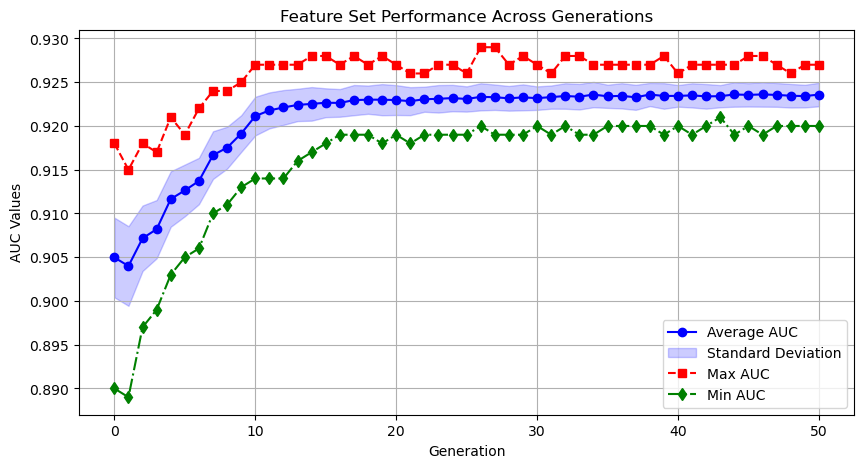

• plot_pso_row_averages will show how the population is improving over time.

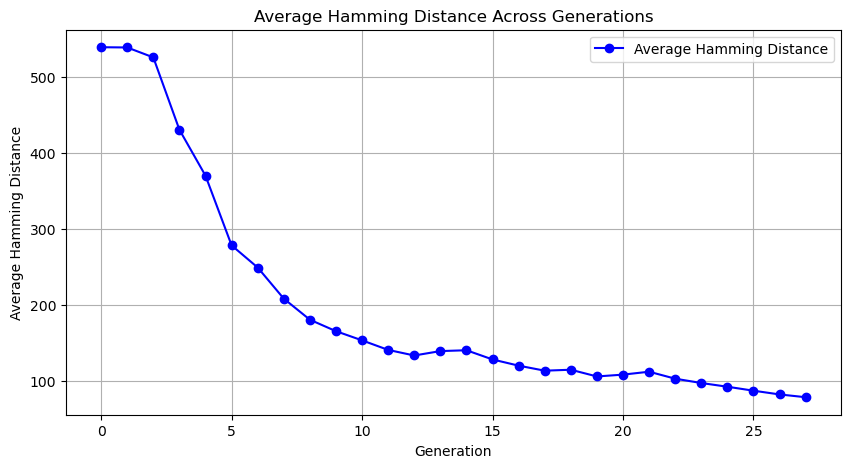
• plot_hamming_distance will track the average Hamming distance between population members, demonstrating the degree of similarity.

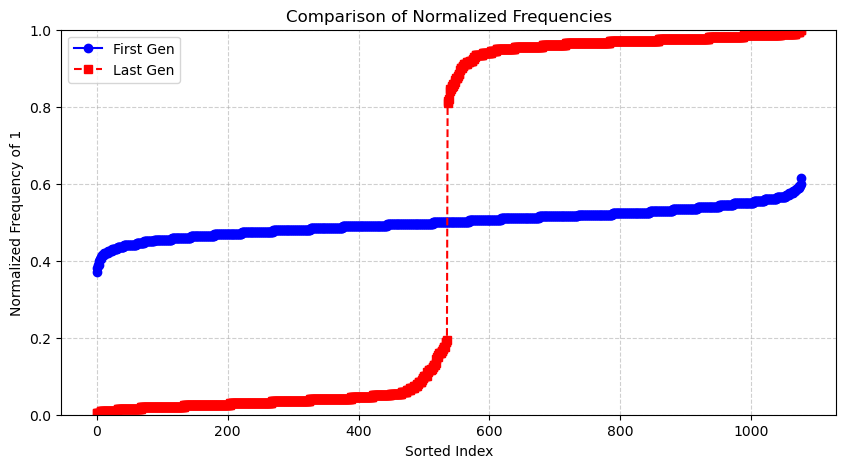
• plot_sorted_frequencies will show the proportional representation of features in the first and latest generations.

The output of the PSO will return the best-performing feature set as well as its associated score. Additionally, the best-performing feature set will be written within the local directory as such: pso_selected_genes.pkl.

Subsequently, you can use the optimized feature set to then train a new model and potentially produce an improved score with regards to the Test set AUC value as such:

with open('pso_selected_genes.pkl', 'wb') as f:
    pickle.dump(pso_genes, f)
      
new_model = PredAnnModel(current_data,pso_genes,num_epochs=50)
ann_plot.evaluate_model(new_model, current_data)

Project Organization

📂 PAGEpy/                         # Source code for the PAGEpy project
├── 📄 PAGEpy_plot.py              # Contains various functions for plotting the data and tracking progress
├── 📄 format_data_class.py        # The FormatData class takes expression data and a target variable to instantiate an object suitable for PSO and training a deep neural network
├── 📄 multiple_folds_class.py     # The MultipleFolds class uses the FormatData class as input to generate multiple folds (default = 5) for cross-validation
├── 📄 indvidual_fold_class.py     # The IndividualFold class generates a single fold which can then be passed directly to the PredAnnModel class
├── 📄 pred_ann_model.py           # Given either the FormatData or IndividualFold the PredAnnModel class instantiates and trains a deep neural network for target variable prediction
├── 📄 pso.py                      # Contains a series of functions for a particle swarm optimization algorithm for feature selection
├── 📄 PAGEpy_utils.py             # Contains various helper functions
📂 example_images/                 # Contains example images for the readme file
📂 example_notebook/               # Jupyter notebooks demonstrating how to process either single-cell or bulk RNA sequencing data sets with PAGEpy
├── 📄 bulk_walkthrough.py         # Bulk RNA sequencing walkthrough
├── 📄 single_cell_walkthrough.py  # Single-cell RNA-sequencing walkthrough
📄 README.md                       # Project description and repository guide
📄 LICENSE                         # MIT license

Function and class descriptions

🔴 FormatData class

A class for preparing and formatting gene expression data for machine learning pipelines.

Initialization

FormatData(
    data_dir='/home/input_data_folder/'',
    test_set_size=0.2,
    random_seed=1,
    hvg_count=1000,
    pval_cutoff=0.01,
    gene_selection='HVG',
    pval_correction='bonferroni'
)

Parameters

• data_dir (str, default='/home/input_data_folder/'): Path to the directory containing necessary input files.
• test_set_size (float, default=0.2): Fraction of the dataset to be used as the test set.
• random_seed (int, default=1): Seed for reproducible dataset splits.
• hvg_count (int, default=1000): Number of highly variable genes (HVGs) to select.
• pval_cutoff (float, default=0.01): Significance threshold for gene selection when using differential expression analysis.
• gene_selection (str, default='HVG'): The method of feature selection, can be either: 'HVG' (Highly Variable Genes) or 'Diff' (Differential Expression)
• pval_correction (str, default='bonferroni'): Method used for multiple hypothesis testing corrections. 'benjamini-hochberg' is another option.

Attributes

• adata (AnnData): Stores single-cell expression data.
• counts_df (pd.DataFrame): DataFrame of raw count data.
• target_variable (array-like): Labels or metadata used for classification.
• x_train, x_test (pd.DataFrame): Training and test feature matrices.
• y_train, y_test (array-like): Corresponding training and test labels.
• genes_list (list): List of all available genes in the dataset.
• selected_genes (list): Subset of genes chosen through HVG or differential expression analysis.
• train_indices, test_indices (array-like): Indices of samples assigned to training and test sets.
• genes (list): Processed gene identifiers.
• barcodes (list): Cell barcode identifiers.
• selected_genes (list): Genes selected through differential expression testing or highly variable gene identification

Methods (Automatically Called)

• self.construct_and_process_anndata(): Constructs the anndata object.
• self.encode_labels(): Binarizes the target variable for training the model.
• self.retrieve_counts_df(): Constructs a counts data frame.
• self.retrieve_all_genes(): Attaches the list of all genes/features to the FormatData object.
• self.scale_data(): Scales and centers the data.
• self.establish_test_train(): Splits the data into test and train sets and performs feature selection using only the training set.

Example Usage

from mymodule import FormatData

# Initialize with custom parameters
data_prep = FormatData(
    data_dir='/path/to/data',
    test_set_size=0.20,
    hvg_count=1500,
    gene_selection='HVG',
    pval_correction='Bonferroni'
)

# Access selected genes
print(data_prep.selected_genes)

🔴 PredAnnModel class

A class for instantiating and training a multi-layer classifier model.

Initialization

PredAnnModel(
    input_data,
    current_genes,
    learning_rate=0.01,
    dropout_rate=0.3,
    balance=True,
    l2_reg=0.2,
    batch_size=64,
    num_epochs=5000,
    report_frequency=1,
    auc_threshold=0.95,
    clipnorm=2.0,
    simplify_categories=True,
    holdout_size=0.5,
    multiplier=3,
    auc_thresholds=[0.6, 0.7, 0.8, 0.85, 0.88, 0.89, 0.90, 0.91, 0.92],
    lr_dict={
        0.6:  0.005,
        0.7:  0.001,
        0.8:  0.0005,
        0.85: 0.0005,
        0.88: 0.0005,
        0.89: 0.0005,
        0.9:  0.0005,
        0.91: 0.0005,
        0.92: 0.0005
    }
)

Parameters

• input_data (FormatData object): Processed dataset used for training, containing gene expression values and labels.
• current_genes (list): A non-empty list of genes used as model features.
• learning_rate (float, default=0.01): Initial learning rate for the model.
• dropout_rate (float, default=0.3): Dropout rate, corresponding to the fraction of neurons that will be randomly inactivated during training, to prevent overfitting.
• balance (bool, default=True): Whether to balance the target variable during mini-batch training.
• l2_reg (float, default=0.2): Strength of L2 regularization, large values add a greater penalty term to the loss function forcing the model to keep the weights small and distributed.
• batch_size (int, default=64): Number of samples per training batch.
• num_epochs (int, default=5000): Maximum number of training epochs.
• report_frequency (int, default=1): Frequency of logging model performance metrics.
• auc_threshold (float, default=0.95): AUC threshold for early stopping.
• clipnorm (float, default=2.0): Maximum gradient norm to prevent exploding gradients.
• simplify_categories (bool, default=True): Whether to simplify data categories before training. (TODO: this is never used?!?-->removed from code)
• holdout_size (float, default=0.5): Fraction of data withheld for training during each training epoch. Reduces the rate of dataset memorization.
• multiplier (int, default=3): Scaling factor for the number of nodes in most layers of the neural network. Large values correspond to a wider network.
• auc_thresholds (list, default=[0.6, 0.7, 0.8, 0.85, 0.88, 0.89, 0.90, 0.91, 0.92]): AUC values at which the learning rate is adjusted. The test AUC value is continuously monitored and the learning rate can change at each of these supplied thresholds in a manner corresponding to the key-value pairs within the lr_dict.
• lr_dict (dict): Dictionary mapping AUC thresholds to corresponding learning rates.

Attributes After initialization, the class contains the following attributes:

• outcome_classifier (keras.Model): The deep learning model for classification.
• test_accuracy_list, train_accuracy_list (list): Accuracy metrics collected during training.
• test_auc_list, train_auc_list (list): AUC values for test and training sets.
• current_epoch_list (list): Tracks epochs where metrics were logged.

Methods (Automatically Called)

• set_mixed_precision(): Enables mixed-precision training for improved performance.
• subset_input_data(): Filters input data based on selected genes.
• build_outcome_classifier(): Constructs the ANN model.
• train_the_model(): Runs the training process.

Example Usage

from mymodule import PredAnnModel, FormatData

# Load and process input data
data_prep = FormatData(data_dir='/path/to/data')

# Define a list of genes to use
selected_genes = ['GeneA', 'GeneB', 'GeneC']

# Initialize and train the model
model = PredAnnModel(input_data=data_prep, current_genes=selected_genes)

# Access model performance metrics
print(model.test_auc_list)

🔴 binary_pso function

Performs feature selection using a Binary Particle Swarm Optimization (PSO) algorithm to optimize a classification model based on gene expression data.

Positional arguments

• current_genes (list): A list of gene names considered for feature selection.
• current_data (pd.DataFrame): A DataFrame containing gene expression values with samples as rows and genes as columns.
• POP_SIZE (int): The number of particles (candidate solutions) in the swarm.
• N_GENERATIONS (int): The number of iterations for the PSO algorithm.

Keyword arguments

• W (float, optional, default=1): Inertia weight controlling the influence of previous velocity on the new velocity.
• C1 (float, optional, default=2): Cognitive coefficient influencing how much a particle follows its personal best position.
• C2 (float, optional, default=1.5): Social coefficient influencing how much a particle follows the global best position.
• reps (int, optional, default=4): The number of times each feature set is evaluated to account for variability.
• verbose (bool, optional, default=False): If True, logs intermediate results more frequently.
• adaptive_metrics (bool, optional, default=False): If True, dynamically adjusts the C1 and C2 values based on observed performance trends. It will decrease C1 and increase C2 when the average population performance is increasing allowing exploitation to take over when a strong solution is found.

Returns

• best_solution (list): The best-performing subset of genes selected.
• best_fitness (float): The highest achieved evaluation metric (e.g., AUC).

Example Usage

best_solution, best_fitness = pso.binary_pso(current_genes, current_data, 100, 20)

📊 Plotting Functions

Several functions are available with the package:

evaluate_model(input_model, input_data)

• Plots model training and evaluation metrics across epochs:

Training and test accuracy with chance level baselines.

Training and test AUC scores.

plot_pso_row_averages(df)

• Visualizes the performance of feature sets across generations: Plots the mean, max, min, and standard deviation of AUC values per generation.

plot_hamming_distance(input_dict)

• Tracks diversity in feature sets over generations: Computes and plots the average Hamming distance among feature sets in each generation.

plot_sorted_frequencies(loaded_dict, loaded_df)

• Compares feature selection frequencies between the first and latest generation: by sorting and normalizing the frequency of selected features between these two generations.

Example Usage

import pandas as pd
import PAGEpy_plot

pso_df = pd.read_pickle("pso_fitness_scores.pkl")
pso_dict = pd.read_pickle("pso_particle_history.pkl")

PAGEpy_plot.plot_pso_row_averages(pso_df)

PAGEpy_plot.plot_hamming_distance(pso_dict)

PAGEpy_plot.plot_sorted_frequencies(pso_dict,pso_df)

🔴 MultipleFolds class

A class for splitting the input data into multiple stratified K-folds. It can be passed to the IndividualFold to access individual K-folds.

Initialization

MultipleFolds(
    input_data,
    folds_count=5
)

Parameters

• input_data (object): An object containing x_train and y_train as pandas DataFrames.
• folds_count (int, default=5): Number of folds for stratified K-fold cross-validation.

Attributes

• x_train_folds (list): List of training feature sets for each fold.
• x_test_folds (list): List of testing feature sets for each fold.
• y_train_folds (list): List of training target sets for each fold.
• y_test_folds (list): List of testing target sets for each fold.
• X (DataFrame): Feature matrix extracted from input_data.x_train.
• y (DataFrame): Target variable extracted from input_data.y_train.
• genes_list (list): List of all genes, extracted from input_data.genes_list.

Methods (Automatically Called)

• get_folds(): Splits the dataset into stratified K-folds and stores the resulting train-test splits.

Example Usage

# Load and prepare input data
data_prep = FormatData(data_dir='/path/to/data')

# Generate stratified folds
folds = MultipleFolds(input_data=data_prep, folds_count=5)

🔴 IndividualFold class

A class to prepare the data for training and testing an Artificial Neural Network using the stratified K-folds from an existing MultipleFolds object.

Parameters

• folds_object (object): An instance of a folds-generating class (e.g., MultipleFolds) containing stratified train-test splits.
• current_fold (int, default=0): The index of the fold to use for training and testing.

Attributes

• folds_object (object): The input folds object storing train-test splits.
• current_fold (int): The index of the selected fold for training and testing.
• genes_list (list): List of genes used for feature selection.
• x_train (DataFrame or ndarray): Gene expression data for the training set.
• x_test (DataFrame or ndarray): Gene expression data for the testing set.
• y_train (DataFrame or Series): Target variable for the training set.
• y_test (DataFrame or Series): Target variable for the testing set.

Methods (Automatically Called)

__repr__(): Returns a string representation of the IndividualFold object, including the current fold index and the shape of unique_combinations_array.

Example Usage

# Generate stratified folds
folds = MultipleFolds(input_data=data_prep, folds_count=5)

# Select an individual fold for ANN training
fold_instance = IndividualFold(folds_object=folds, current_fold=2)

License

This project is licensed under the MIT License - see the LICENSE file for details.

Contact

For any questions or suggestions, reach out to:

• Sean O'Toole - [email protected]
• GitHub: sean-otoole

---