The Compact Muon Solenoid (CMS) is a detector at the Large Hadron Collider (LHC) located near Geneva, Switzerland. The CMS experiment detects the resulting particles from the collusion and measures their kinematics using various sub detectors working in concert. High momentum muons are significant objects for many physics analyses at CMS. Therefore, an accurate momentum assignment scheme differentiating low momentum muons (background) from high momentum muons (signal) is crucial to the Endcap Muon Track Finder (EMTF) trigger. The first algorithm implemented in the trigger system was a discretized boosted decision tree. In this work, we study the use of deep learning algorithms (Fully Connected Neural Networks (FCNNs), Convolutional Neural Networks (CNNs) and Graph Naural Networks (GNNs)) at the trigger level that requires highly optimized inference. We develop and benchmark the GNNs for momentum regression in the trigger system.
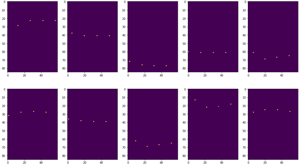
Codes used to train and test the models are available under Models folder. Training results for FCNN and CNN models can be found in GSoC v5.ipynb and GSoC v6.ipynb. The difference between two scripts is the generation of 2D images for the CNN model. In the former, Phi angle, Theta angle and Front/Rear hit features are used to locate exact locations of the hits in 4 detectors as follows:
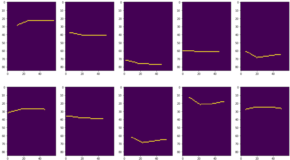
Then, linear interpolation is utilized to obtain the complete trajectory of the muons as below:
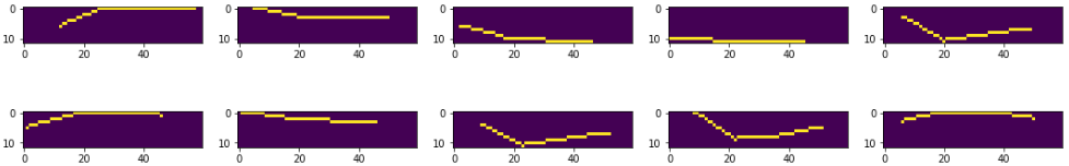
Since a great part of the images are empty, they introduce redundancy in the feature space. To eliminate this problem, we crop the generated images while keeping the whole trajectory within the bounds as follows:
In the latter, on the other hand, we use all the features (Phi Angle, Theta Angle, Front/Rear Hit, Bending Angle, Time, Mask, Ring Number) to generate 2D images as follows:
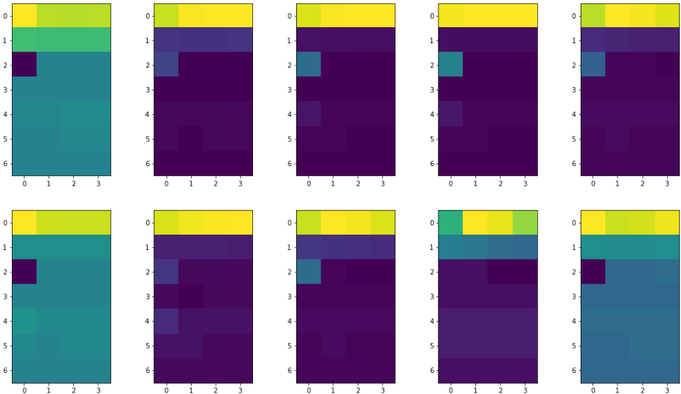
Although these images are not as intuitive as in the previous method, they contain much more information due to larger feature space. In the former method while we obtained losses of 0.025 and 2.0125e-04 for pT and 1/pT prediction, respectively, in the latter one, we achieved losses of 0.01 and 7.3357e-05. Therefore, in the remaining benchmarkings of the study, the latter image generation method is used.
Codes for different GNN models are also presented under Models, and complete comparison of the created models with various metrics (i.e. mean absolute error, accuracy and F-1 score) are available in Compare Models Predictions.ipynb. results folder contains the predictions (.csv files) for the testing dataset used to benchmark the models. An intuitive comparison of the GNN models and their performances are available in this blog post.
Should you have any questions, please contact me at ekurtoglu@crimson.ua.edu