Week 1 - Introduction and Simple C++ Concepts

What is an Algorithm

An algorithm is a well defined computational process that takes some input and produces and output

What is a Data Structure

A data structure is a way to store and organise data. It can also be seen as a special type of algorithm.

Strings

• Strings in C are null terminated char arrays.
• In C++ there is an added implementation of a proper string class (std::string) that acts as a wrapper for char[], as well as fixing issues when dealing with null termination

Null Pointers

• In C++ a null value is actually just 0 (or something that looks like it)
• Since C++11 an actual null_ptr type exists, which means you're able to have a proper null (similar to C) that isn't just 0.

Memory Allocation

Static Allocation

• Declaring a static variable is usually placed onto the stack (usually*).
• The variable will die at the end of the code block in which it is defined (they will be automatically deallocated).

Dynamic Allocation

• Dynamically allocating a variable will be usually placed onto the heap (usually*).

• C++ does not contain any garbage collection, which means the variable will no longer be automatically deallocated, and you will have to decide where to deallocate it using the delete keyword.

• BIG MUST: The delete MUST be used if you dynamically allocate memory.

int* arr = new int[5];
[...]
delete[] arr; // delete[] is used for arrays

[*] NB: C++ Standard does not specify where to allocate dynamic or static memory

Arrays

Arrays in C++ are very similar to Java arrays:

int a[4] = {1,2,3,4};
int a[] = {1,2,3,4};
int a[4] = {};
int a[4];

Arrays are statically created, which means they will automatically deallocate once out of scope. However, one thing to note is that C++ arrays need a size to be declared. If we don't know the size of the array to use, we can use a pointer:

• Arrays can be treated as pointers e.g. int[] = int*
• Technical jargon: Arrays decay to pointers to the first element of the array.

Pointers

A pointer is an object that refers to another object

double* px; // initialise a pointer
double x = 5.1234
px = &x;   // setting a pointer to the memory address of an object
*px; // obtains the value pointed to by the pointer (dereferencing)
(*px).bar = px->bar // arrow notation can be used to access a member

References

A reference variable is used to give a name to an object. It refers to the same object. For Example:

int& rx = x;

• the reference variable rx references x, which means that if you change the value of rx, it will also change the value of x.

Using references is extremely useful for when passing a value into a function by reference:

void do_something_cool(int& x) {
	x = x + 1;
}
int y = 1;
do_something_cool(y); // y now equals 2

Classes

Class myClass : public parentClass {
private: 
	int private_int;
public:
	int getPrivateInt();
	void setPrivateInt(int value);
	string toString();
}

C++ Separates definitions from source code:

• Definitions are placed in a header file (.h, .hpp etc.)
• Source Code is in source files (.cpp etc.)
• Code can also be placed entirely in the header file

Abstract Data Types / Linked List virtual Class example

Abstract data types don’t specify implementations, rather they are just specifications of behaviour of Data Types (Same as an interface and abstraction)

Class intList {
public: 
	virtual ~intList() {};
	virtual bool isEmpty() = 0;
	virtual void prepend(int c) = 0;
	virtual int head() = 0;
	virtual intList tail() = 0;
}

Week 2 - I/O, Destructors, Stacks, Queues

cin and cout

int n;
std::cout << “Enter a number!” << std::endl();
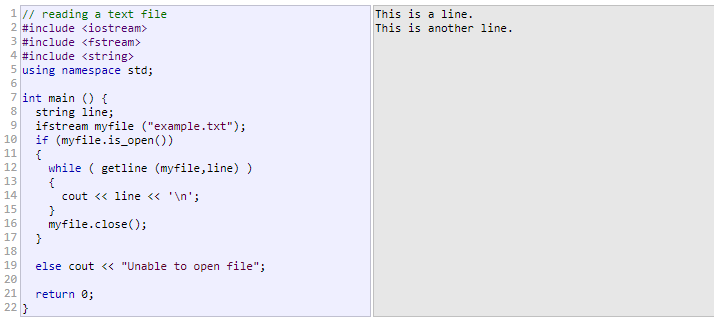
std::cin >> n;

To get an entire line:

std::getline(std::cin, [variable to read into]); std::err can be used to output errors

File I/O

Destructors

e.g. ~intLinkedList()

Destructors are a special method that is run when an object has the special delete operator called on it

delete [pointer to thing to delete]
delete[] [array variable] // because arrays are a pointer, so this works the same way

The delete is required when we've created something with new. Otherwise heap memory is not deallocated, and we have a memory leak.

Exceptions

C++ has a try/catch implementation

try {
	throw 20;
} catch (int e) {
	// print error here
}

Compiling with multiple files

• Just list all other cpp files after the main.cpp g++ main.cpp other.cpp etc.cpp
• can also use g++ *.cpp -o output

Queue

• A FIFO (First-in-first-out) data structure
• Can only be added to the back
• Can only be taken off the front
• Unbounded capacity (normally)

class intQueue {
public:
	virtual ~intQueue() {};
	virtual void enqueue(int n) = 0;
	virtual int dequeue() = 0;
	virtual int peek() = 0;
};

Other Queues

• A Deque (double-ended queue). Can add and remove at both ends
• Priority Queue is a queue, but elements are inserted with a priority, and come out in priority order.

Stacks

• A LIFO (Last-in-first-out) data structure
• Add from the top
• Remove from the top

class intStack {
public:
	virtual ~intStack() {};
	virtual void push() = 0;
	virtual int pop() = 0;
	virtual int peek() = 0;
}; 

Week 3 - Vectors, Templates, Iterators, Big-Oh

Vector Class

std::vector<T>

• Arrays are hard to manage in C/C++. Vectors are a good alternative to this, and can be seen as dynamically size arrays.
• Has element access: at, operator[], front back etc.
• Has iterators! begin -> end, cbegin -> cend, rbegin -> rend, crbegin -> crend
• Can be checked for its capacity: empty, size, max_size etc.

Templates

• A good way to write certain types of code once, if the code doesn't care about the types it is working with
• We can make a std::vector<int>, or even a std::vector<char>. Within classes:
• Make sure to add a template <typename T> before using templates within a class

template <typename T> 
class node {
  private:
    T data;
    node *next;
}

Iterators

An iterator is any object that, pointing to some element in a range of elements (such as an array or a container), has the ability to iterate through the elements of that range using a set of operators (with at least the increment (++) and dereference (*) operators).

The most obvious form of iterator is a pointer: A pointer can point to elements in an array, and can iterate through them using the increment operator (++). But other kinds of iterators are possible. For example, each container type (such as a list) has a specific iterator type designed to iterate through its elements.

Asymptotic Notations

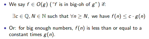
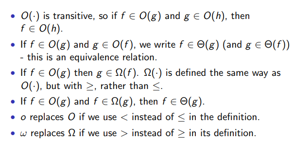
• O (Big-Oh) Notation: The upper bound of an algorithm
• Θ (Theta) Notation: Bounds a function from above and below, defines exact asymptotic behaviou
• Ω (Omega) Notation: Asymptotic lower bound

Big-Oh Notation

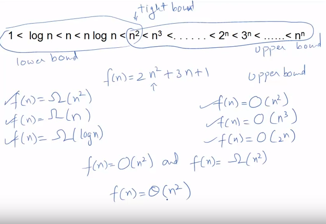
Comparing two functions f and g:

• This helps us as we can now compare and decide which function is the fastest (in its worst case scenario)
• "One of the algorithm's running time will be larger for large enough inputs"

Big-Oh Rules

Big-Oh Names

How to get the functions

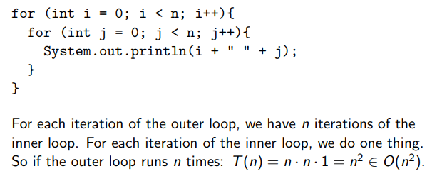
Count the number of steps

Other Properties

Week 4 - Divide and Conquer, Recursion, Iteration

Divide and Conquer

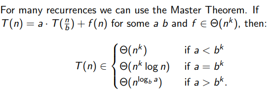
The general framework for a divide-and-conquer algorithm is:

1. Divide the instance into a set of sub-problems
2. If a subproblem is small enough, solve it, otherwise recursively split the subproblem
3. Combine the subproblem solutions into a whole solution.

Examples of Divide and Conquer - Binary Search

finds if an element is in a sorted array (probably the simplest d&c algorithm, and is in O(log n) time):

1. Check the middle of the array, is the middle greater or smaller than the target element?
2. If it’s the same, you’ve found it! If the array is size one and it’s not the same, it’s not there!
3. If it’s greater, search the left side of the array. Otherwise search the right.

Examples of Divide and Conquer - Exponential

int exp(x, n) {
	if (n == 0) then
		return 1;
	if (n%2) // if is odd
		return x * exp(x, n-1);
	else {
		int y = exp(x, n/2);
		return y * x; 
	}
}

Master Theorem

Recursion

Recursion is conceptually a central component of Divide & Conquer. Recursion can lead to "neat" code, however will also lead to inefficient and broken code.

Designing a Recursive Algorithm

Carefully specify:

1. The Preconditions: what must be true about the input before you start the algorithm.
2. The Post-conditions: what must be true about the output when you’re done.

These conditions then apply at every step of the recursion.

Work out how to measure the “size” of an instance.

Consider a general instance of the problem:

1. Imagine you have friends who can magically solve any instance of the problem strictly smaller than yours if it meets the preconditions.
2. From your instance, construct sub-instances that meet the preconditions.
3. Get your friends to solve them.
4. Recombine the sub-solutions.

Recursion vs Iteration

• Recursion often gives nice "simple" algorithms, but making them efficient can be trickier
• Iterative algorithms are often easily made efficient (and easily optimised by compilers), But they result in hard-to-understand code.

There is not always a simple answer to which one to used, both approaches can be used, and you must think about what works best for the problem.

Things to consider when choosing

1. Is my problem naturally recursive or iterative?
2. Do I know how to terminate the algorithm (base cases for recursion, loop conditions for iteration)?
3. Will I re-use the same information over and over?
   • A candidate for memoization - recursion, but where we remember what we’ve already calculated.
   • If memoization isn’t good, then this should probably be iterative.
4. Are the limits well defined (not just can I guarantee they will be met, but do I know them in advance)¿
   • If not, recursion will probably be easier.
5. Can I do it tail-recursively?
   • Has only one recursive call, at the end of the function - this is often easy to read, but the compiler can also optimise it into iteration.

Week 5 - Graphs Part 1

Graphs

Graphs are an incredibly useful modelling tool. Simple graphs consist of:

• A set of elements called vertices.
• A set of unordered pairs of distinct vertices called edges.
• There is only one edge between a pair of vertices.

Other types of graph come from altering these conditions:

• Ordered pairs gives directed graphs.
• More than one edge per pair gives multi-graphs.
• More than two vertices per edge gives hypergraphs.
• Edges (and vertices) can be weighted, labelled, &c.

Graphs Applications in Real Life

Vertices within graphs model many things such as:

• Computers
• Processes
• Proteins
• Production facilities
• Websites

Edges model relationships between the things:

• Network links
• Shared resources
• Protein interactions
• Transport links
• Hyper links

Notation and Definitions

Adjacency: If two vertices have an edge between them, they are adjacent Incident: If a vertex is one of the pair that forms an edge, it is incident to that edge. Degree: The number of edges incident to a vertex is the degree of that vertex. Arcs: Directed edges

When denoting graph components:

• Graphs will be denoted with uppercase letters like G, H, &c.
• Vertices will be denoted by lowercase letters like u, v, &c., or natural numbers 1, 2, 3, 4, . . . , n.
• Edges will be denoted by lowercase letters like e, d, &c. or by their incident vertices:
  • In undirected graphs uv.
  • In directed graphs (u, v) – u is the tail, v is the head.
  • Directed edges are also called arcs.

Basic Operations

• addVertex(Vertex v)
• removeVertex(Vertex v)
• addEdge(Vertex u, Vertex v)
• removeEdge(Vertex u, Vertex v)
• adjacent(Vertex u, Vertex v)
• degree(Vertex u)
• return the vertices in the graph
• return the edges incident to a vertex
• return the vertices adjacent to a vertex

Graphs as Data Structures

Adjacency Matrix

Quick access – O(1), but with not so great space and set-up – O(n^2) (with n vertices).

The simplest form:

• Edges are stored as a two-dimensional matrix (e.g. vector<vector<bool> > edges or bool edges[][]
• if edge[i][j] == true, then vertex i is adjacent to vertex j.

Some enhancements:

• can use a numeric (int,double) matrix to give weighted edges.
• Can use a matrix of Edges if edges are more complex – a null-type value means no edge.
• Easily supports directed graphs and undirected graphs.
• If vertices have associated data, we can store them separately (another array would make matching indices easy).

Adjacency List

• Each vertex has associated with it a list of its adjacent vertices.
• Could be a size n array of linked lists, or similar.
• Slower to determine adjacency – O(n), but faster to return all adjacent vertices – O(1).
• Most compact space representation O(m + n) where m is the number of edges in the graph – we have to store something for each vertex and edge anyway, so this is the best we can do.
• Easy to modify for more complex edge and vertex data structures.
• Works best for sparse graphs (few edges per vertex).

Object Oriented Approach

• We have classes for Vertex, Edge and Graph.
• Vertex contains a list of its Edges.
• Each Edge knows its endpoints.
• the Graph knows about everything.
• Lots of references to keep track of.
• Tends to be the slow way to do things, but has a nice match to the conceptual version.

Traversing Graphs

Depth First Traversal

• Pick a starting vertex.
• Recursively pick an unvisited neighbour and visit it.
• Can be implemented recursively, or iteratively using a stack.

Recursive:

dft(Vertex v){ 
	mark v as visited; 
	visit(v); 
	for each neighbour u of v { 
		if (u is unmarked) 
			dft(u); 
	} 
}

Iterative:

dft() { 
	pick starting vertex v; 
	Stack unprocessed = new Stack(); 
	unprocessed.push(v); 
	while (!unprocessed.isEmpty()) { 
		Vertex u = unprocessed.pop(); 
		if (u is unmarked) { 
			visit(u); 
			mark u; 
			for each neighbour w of u { 
				unprocessed.push(w); 
			} 
		}
	} 
}

Breadth First Traversal

• Pick a starting vertex and put it in a queue.
• Iteratively take a vertex from the queue, visit it and place all its neighbours in the queue.
• It’s inherently iterative, it’s not impossible to implement recursively, just silly.

bft() { 
	pick starting vertex v; 
	Queue unprocessed = new Queue();
	unprocessed.offer(v); 
	while (!unprocessed.isEmpty()) { 
		Vertex u = unprocessed.poll(); 
		if (u is unmarked) { 
			visit(u); 
			mark u; 
			for each neighbour w of u {
				unprocessed.offer(w); 
			} 
		} 
	} 
}

Breadth First vs. Depth First

• Some graphs produce the same traversal order for both.
• Which one to use will depend upon the application.
• Notice the iterative versions of both are actually identical – just swap the stack and the queue.
• Both O(n + m).

Greedy Algorithms

Greedy Algorithms are based on picking what looks good now.

• One of the simplest algorithmic paradigms.
• Usually easy to implement.
• Only really works for certain types of problems.
• For some problems, a greedy approach may produce the worst solution!

Greedy Algorithms usually work when the problem satisfies two properties:

• Optimal Substructure: Optimal solutions contain optimal subsolutions to subproblems (you can split solutions up and they’re still good).
• Greedy Choice Property: Any decisions depend only on what you’ve already seen (you don’t have to come back and fix things).

Spanning Trees of Graphs

Spanning Tree Terms

Subgraph: A subset of the vertices and the edges of a graph that form a graph Spanning: A graph is spanning if it includes all the vertices of the original graph Spanning Tree: A spanning subgraph is a spanning tree if it contains no cycles. Minimum Spanning Tree: a minimum spanning tree if it has minimum total (edge) weight over all possible spanning trees of that graph (is it unique?).

• In unweighted graphs (or a graph where all edge weights are the same), any spanning tree is a minimum spanning tree.

• We can compute one from a depth-first or breadth-first traversal.

• If we have different weights on the edges, a simple traversal is not enough.

• There are two main algorithms: Prim’s Algorithm and Kruskal’s Algorithm

Prim's Algorithm

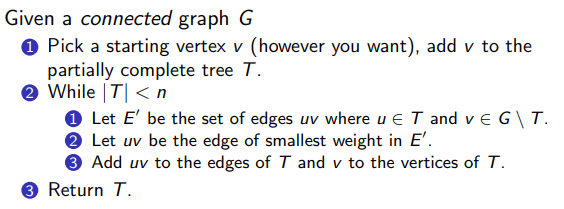
1. Keep track of which edges and vertices are in the tree.
2. Pick the next smallest edge that extends the tree, add it.
3. Keep going until the whole graph is spanned.

Algorithm Complexity:

• If we use an adjacency matrix O(n^2)
• Putting edges into a binary heap, with the graph sorted as an adjacent list O((n+m)log n) = O(mlog n)

Kruskal's Algorithm

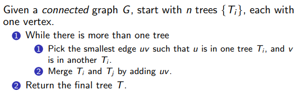
• e.g. Start with a lot of trees (a forest), and pick the best edge to connect two components (trees) together, until the whole thing has been connected

Algorithm Complexity:

• By labelling vertices with which component they’re in, we can get O(n · m) – not great.
• If we sorted the edges, and employ an efficient disjoint set data structure: O(m log m) = O(m log n) – about the same as the normal Prim implementation.
• If the edges can be sorted efficiently by counting sort or radix sort or similar, we can get O(m · α(n)), where α(n) is the inverse of the single valued Ackermann function.

Borůvka’s Algorithm

Is kind of like a cross between Prim's and Kruskal's.

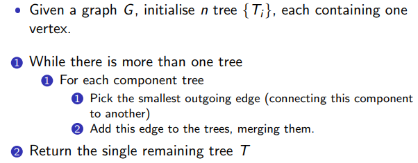
Algorithm Complexity:

• The outer loop only needs to execute O(log n) times – we halve the number of components at each step.
• Along with search for the edges at each iteration, we get O(m log n) without too much fiddling.
• A similar approach as used for Kruskal’s can be used to get O(m · α(n)).
• A randomised version exists with O(m) expected running time – remember this is linear in the size of the graph, about as fast as possible.

Spanning Trees and Disconnected Graphs

• If the graph has several disconnected components, we can’t get a spanning tree (trees have to be connected).
• We can get a spanning forest.

Reverse-Delete Algorithm

• Appears the same as Kruskal's algorithm, sort of like a backwards Kruskal's
• Removes edges instead of adding them, to determine what we're left with at the end

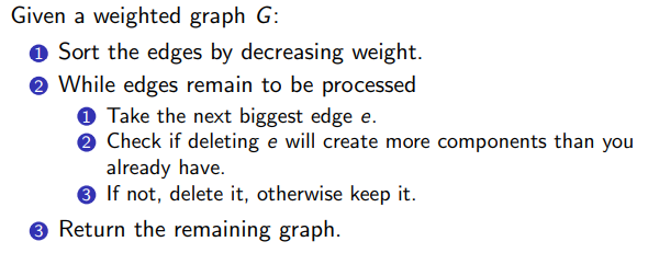
Algorithm Complexity:

• We can sort the edges in O(m log m).
• We can check the connectivity in O(log n(log log n) 3 ).
• So in total we get O(m log n(log log n)^3 ) time

Week 6 - Binary Trees

Binary Tree

Tree: is a graph with no cycles e.g. you can't walk through the graph and get back to the starting point without backtracking Binary Tree: A tree where every vertex has at most three neighbours:

• One vertex is the root
• Each vertex has at most two children, and at most one parent
• Vertices with no children are called Leaves

Uses of Binary Trees

• 3D rendering (binary space partition).
• Networking (Binary Tries, Treaps).
• Cryptology (GGM Trees).
• Coding and Compression (Huffman Trees).
• Hashing (Hash Trees).
• Sorting (Heaps and Heapsort).
• Searching (Binary Search Trees).
• Parsing (Expression Trees)

How to Create Binary Trees

Either:

1. Create a type of linked list, but instead of one next pointer, you add a second pointer to accommodate for both left and right children
2. Embedded within an array, where the children of the vertex at index i are at indices 2i and 2i+1

Depth First Traversal

Very amenable to recursive implementation:

• At each node we have 3 things to do:
  1. Deal with the current node,
  2. visit the left child,
  3. visit the right child.
• Gives 3 different traversals.
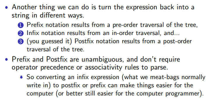
  • Pre-order (deal with the current node first)
  • In-order (deal with the current node between visiting the descendents)
  • Post-order (deal with the current node last).

Recursive implementations

All 3 are the same, except that you change where the visit(n); code block is placed

recursiveTraversal(Node n) { 
	if (n == null) return; 
	visit(n); // pre order only
	preorderTraversal(n.leftChild());
	visit(n); // in order only 
	preorderTraversal(n.rightChild()); 
	visit(n); // post order only
}

Pre-order iterative

preorderTraversal(Node n) { 
	Stack s = new Stack(); 
	Node current = n; 
	while (current != null) { 
		visit(current); 
		if (current.rightChild() != null) 		
			s.push(current.rightChild()); 
		if (current.leftChild() != null) 
			s.push(current.leftChild()); 
		
		current = stack.pop(); 
	} 
}

In-order iterative

inorderTraversal(Node n) { 
	Stack s = new Stack(); 
	Node current = n; 
	while (current != null || !s.isEmpty()) { 
		if (current != null) { 
			s.push(current); 
			current = current.leftChild(); 
		} else { 
			current = s.pop(); 
			visit(current); 
			current = current.rightChild(); 
		} 
	} 
}

Post-order iterative

postorderTraversal(Node n) { 
	Stack s = new Stack(); 
	Node current = n; 
	Node last = null; 
	while (current != null || !s.isEmpty()) { 
		if (current != null) { 
			s.push(current); 
			current = current.leftChild(); 
		} else { 
			if (s.peek().rightChild() != null && 
				s.peek().rightChild() != last) { 
				current = s.peek().rightChild(); 
			} else { 
				current = s.pop(); 
				visit(current); 
				last = current; 
			} 
		} 
	} 
}

Breadth First Traversal

• Visits vertices according to their level in the tree (left to right, top to bottom).
• Use a queue to simply implement iteratively

breadthFirst(Node n) { 
	Queue q = new Queue(); 
	q.add(n); 
	while (!q.isEmpty()) { 
		Node current = q.remove(); 
		visit(current); 
		if (current.leftChild != null) 
			q.add(current.leftChild()); 
		if (current.rightChild != null)
			q.add(current.rightChild()); 
	} 
}

Binary Search Trees

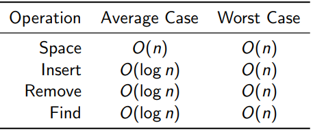
• A Simple data structure that allows fast insertion, removal and lookup of the elements they store.
• They are an ordered data structure, but because they use a binary tree, you don’t have to reshuffle everything to put something new in (compared to array-like data structures).
• Rule of implementation: If what you’re looking for (or what you have) has a smaller key than the current vertex, go to the left. Otherwise, go to the right. (Special case: duplicate keys)
• Insertion involves traversing the tree to the bottom and adding a new element where you stop

Uses of Binary Trees

• Grammar trees
• Boolean Expressions
• Very useful for compiling code (and operation precedence)

Prefix, Infix and Postfix