A Computational Soap Box Slide

This Python package is written by Toon Verstraelen for students of the course "Python for Scientists" (C004212) of the B.Sc. Physics and Astronomy at Ghent University. It is distributed under the conditions of the GPLv3 license.

Quick Start

You can install the soapboxslide Python module with:

pip install soapboxslide

This module implements a 2D surface that resembles a curved slide, suitable for computational soapbox racing. To give you a quick idea, the following figure is created with the plot.py script in this repository, and visualizes the slides boxcar_blitz.toml and brutal_bends.toml included in this repository:

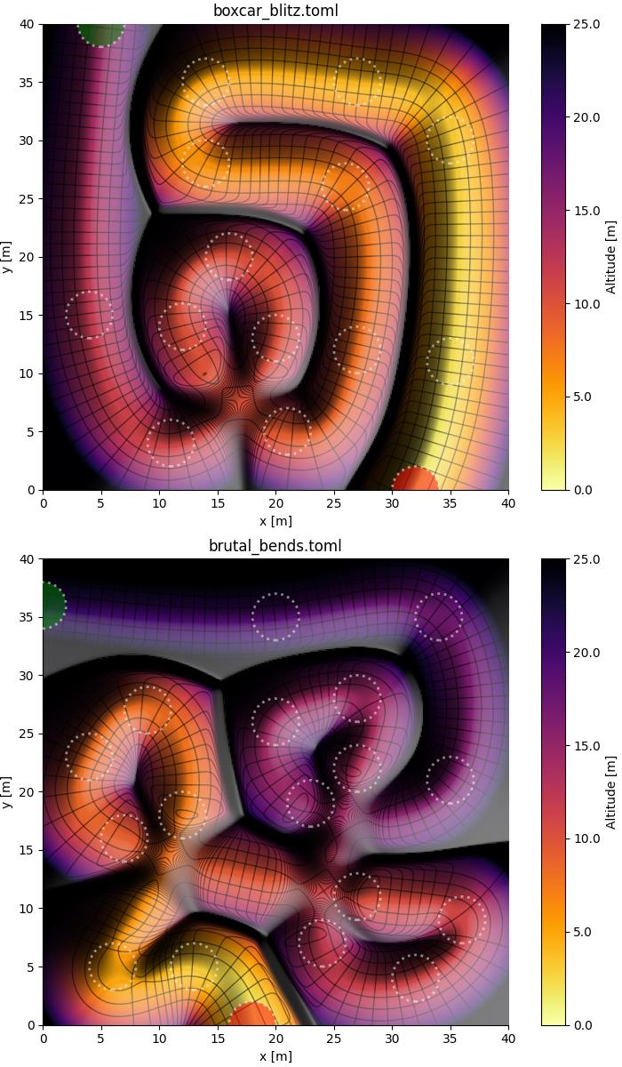
Your eyes may need some time to adapt to the correct depth perception: black ridges are high-altitude separations between the colored valleys.

Note that the starting point and the finish are denoted as green and red circles, respectively. All other circles are waypoints that must be visited on the way down.

Concept

The idea is for students to use the surface implemented in soapboxslide to simulate the dynamics of a particle (or a connected set of particles) sliding down. In addition to correctly implementing the dynamics, students are instructed to find the physical parameters for which the point mass(es) to reach the final target as quickly as possible, without missing any of the intermediate waypoints.

Two classes of physical models can be considered:

1. The most convenient is to assume a model of point particles strictly bound to the surface with holonomic constraints. In this case, equations of motion can be derived using a Lagrangian, possibly with a generalized force to include non-conservative friction forces.

2. A more challenging scenario (not used for now, but closer in spirit to real soap box races) is to impose inequality constraints, allowing particles to fly over the surface.

Slide Class Usage

You can load a slide surface from a TOML file and calculate slide properties at a given point, e.g. $x=5$ and $y=38$, as follows:

import numpy as np

from soapboxslide import Slide

slide = Slide.from_file("boxcar_blitz.toml")
print(slide(np.array([5.0, 38.0])))

This will show three results:

(array(2.05331579), array(0.20172586), array(14.75904983))

These three values have the following meaning (in meter):

1. The progress along the track.
2. The orthogonal(ish) deviation from the bottom of the track.
3. The altitude of the track.

The slide() function is fully vectorized: one may also provide an array of points to calculate many altitudes efficiently. (This is useful for plotting.)

The slide() function optionally supports alternative NumPy wrappers, such as those of JAX and its predecessor Autograd. This allows for an efficient evaluation of analytical partial derivatives of the altitude. For example, a vectorized calculation of many gradients is implemented as follows:

from functools import partial

import jax
import jax.numpy as jnp
import numpy as np

from soapboxslide import Slide

# We recommend double precision:
jax.config.update("jax_enable_x64", True)

# Define the slide and its gradient
slide = Slide.from_file("boxcar_blitz.toml")
alt_grad = jax.jit(jax.vmap(jax.grad(
    lambda pos: slide(pos, npw=jnp)[2]
)))

# Compute the gradient at several points
pos = np.array([
    [5.0, 38.0],
    [12.1, 7.3],
    [10.7, 25.5],
])
print(alt_grad(pos))

This will show three gradients, one for each row of pos:

[[ 0.21289734  0.10176584]
 [-1.85311237  1.84445056]
 [-2.16704263 -2.9280058 ]]

In addition, a Slide instance has the following attributes:

• width: the width of the slide arena in meter.
• height: the height of the slide arena in meter.
• waypoints: A 2D NumPy array with three columns (and at least two rows) defining the shape and altitude of the slide track. These are also intended as points that must be visited by a particle or a system sliding down, to ensure that it followed a legitimate trajectory.
• target_radius: a required proximity between a particle (or the center of mass of a system of particles) to a waypoint, to mark this waypoint as properly visited. The distance is only measured in the $xy$-plane.

Note that the above surface plots show dashed circles centered on the waypoints, whose radius is the target radius.

The Slide class also features two potentially useful methods:

• Slide.get_hits can be used to check which waypoints were reached by a given trajectory.
• Slide.plot can be used to prepare a drawing of the slide on which one can overlay additional results. It supports several keyword arguments to customize the surface.

This is a minimal example using the Slide.plot method, to which one can easily add more matplotlib code:

import matplotlib.pyplot as plt

from soapboxslide import Slide

# Prepare plot with slide surface
slide = Slide.from_file("boxcar_blitz.toml")
fig, ax = plt.subplots(figsize=(8, 7))
slide.plot(fig, ax)

# Customize plot
ax.set(title="You can put here whatever you want")
ax.plot([5.0, 20.0, 9.0], [36.0, 1.0, 5.0], "g-", lw=4)

# Save
fig.savefig("myplot.jpg")

Consult the docstrings for more information on how to use the get_hits and plot methods.

Storing and Sharing Trajectory Data

The soapboxslide module also implements a Trajectory class for storing the results of a numerical integration of one or more particles sliding over the surface. This class performs an initial validation of the trajectory data upon construction. It also features to_file and from_file methods with which trajectories can be dumped to and loaded from NPZ files. This is useful if you want to share your trajectory with someone, e.g. for review, and to implement separate computation and visualization scripts (or notebooks).

To use the Trajectory class, create an instance as follows after completing the numerical integration of the equations of motion:

traj = Trajectory(
    time=...,        # NDArray[float], shape = (ntime, )
    mass=...,        # NDArray[float], shape = (npoint, )
    gamma=...,       # NDArray[float], shape = (npoint, )
    pos=...,         # NDArray[float], shape = (ntime, npoint, 3), (x, y and z coordinates)
    vel=...,         # NDArray[float], shape = (ntime, npoint, 3), (x, y and z coordinates)
    grad=...,        # NDArray[float], shape = (ntime, npoint, 2), (h_x and h_y derivatives)
    hess=...,        # NDArray[float], shape = (ntime, npoint, 3), (h_xx, h_xy and h_yy derivatives)
    spring_idx=...,  # NDArray[int], shape = (nspring, 2), (each row is a pair of point indexes)
    spring_par=...,  # NDArray[float], shape = (nspring, 3), (force constant, rest length, damping coeff)
    end_state=...,   # One of the EndState enumeration
    stop_time=...,   # Optional, time that last target was reached
    stop_pos=...,    # Optional, NDArray[float], shape = (npoint, 3), positions at stop time
    stop_vel=...,    # Optional, NDArray[float], shape = (npoint, 3), velocities at stop time
)
traj.to_file("traj.npz")

In this Python snippet, you need to replace all triple dots by arrays you defined or computed. Some guidelines:

• If there are no springs yet, use arrays with zero rows for the spring definitions.
• If there is just one particle, several arrays will have a size 1 axis, i.e. npoint=1.
• You can first store all fields in a dictionary, e.g. data = {"time": ..., ...} and optionally add the stop_* fields to the dictionary. The trajectory is then created with Trajectory(**data).
• The end state can be specified to indicate when the numerical integration has ended, using one of the EndState instances defined in the soapboxslide module:
  • EndState.STOP: last target was reached in time.
  • EndState.CRASH: the numerical integration failed (e.g. due to Inf or Nan results).
  • EndState.FAR: the particle moved more than 5 m out of the arena.
  • EndState.TIMEOUT: the maximum time, e.g. 60 s, was reached.
• When creating a Trajectory instance, you will get a TypeError or ValueError if some of the data do not meet basic expectations.

The meaning of and requirements for all attributes is further elaborated in the docstrings in soapboxslide.py.