Module 1

Neuron and Neural Networks Weight initialization Activation functions Loss functions Backpropagation Dataloaders Metrics Overfitting and underfitting

1.1 Introduction to Deep Learning

What is Deep Learning?

Artificial Intelligence (AI), Machine Learning (ML), and Deep Learning (DL) are foundational concepts in modern computer science. Although often confused, they are not the same. They are distinct concepts that form a clear hierarchy: Machine Learning is a subfield of AI, and Deep Learning is a specialized branch of Machine Learning.

Machine learning includes straightforward methods such as linear regression and decision trees as well as more sophisticated techniques like random forests and support vector machines. These approaches are generally easier to interpret than deep learning. Deep learning uses artificial neural networks with many layers to model complex patterns. These networks, inspired by the human brain’s structure, excel at learning from large volumes of data.

Its importance

Deep learning has become a cornerstone of modern artificial intelligence because it can automatically discover intricate patterns in data without manual feature engineering. By stacking many layers of artificial neurons, deep learning models learn hierarchical representations, ranging from simple edges in images to abstract concepts such as faces or objects, and enable breakthroughs in computer vision, natural language processing, and beyond.

Deep learning scales effortlessly on large datasets and takes full advantage of modern hardware such as GPUs and TPUs. It transforms raw inputs like images, text and audio into meaningful insights that power real-time speech recognition and machine translation with near-human accuracy. In healthcare, it enables medical image analysis that can detect diseases earlier than radiologists, and in transportation, it drives autonomous vehicles capable of navigating complex environments. Wherever data is abundant and patterns are subtle, deep learning unlocks innovation, pushes performance boundaries and opens possibilities that were unimaginable just a decade ago.

Applications

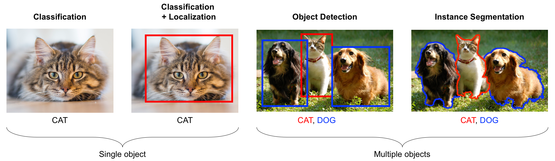
• Computer Vision

  • Object Detection: Amazon uses object detection in its fulfillment centers to scan shelves and identify products in real time, speeding up order picking and reducing stock-out errors.
  • Image Classification: Google Photos applies image classification to automatically tag and organize users’ photos by detecting people, places and objects.
  • Semantic Segmentation: Tesla’s Autopilot segments road scenes into drivable lanes, sidewalks and obstacles, enabling more precise path planning for autonomous driving.
  • Medical Imaging Analysis: DeepMind’s retinal screening system classifies eye scans to detect signs of diabetic retinopathy earlier and more reliably than standard clinical assessment.

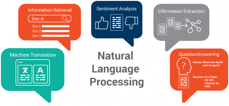
• Natural Language Processing (NLP)

  • Machine Translation: DeepL and Google Translate use transformer-based models to translate text between dozens of languages with near-human fluency.
  • Text Summarization: OpenAI’s GPT-based APIs summarize long articles into concise abstracts, helping researchers and professionals digest information quickly.
  • Sentiment Analysis: Twitter employs sentiment analysis to monitor public opinion by classifying tweets as positive, negative or neutral in real time.
  • Question Answering: IBM Watson’s NLP models power customer-service chatbots that interpret user queries and retrieve exact answers from large knowledge bases.

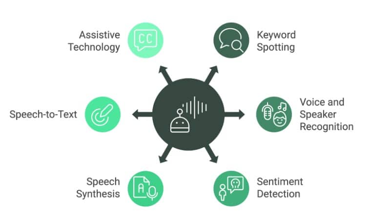
• Speech

  • Automatic Speech Recognition (ASR): Apple’s Siri and Amazon Alexa convert spoken commands into text with high accuracy, enabling hands-free device control and information retrieval.
  • Text-to-Speech (TTS): Google’s WaveNet generates natural, human-like speech from text for use in virtual assistants, audiobooks and accessibility tools.
  • Speaker Identification: Banking apps use speaker identification to verify a caller’s identity by matching voice prints against enrolled profiles, strengthening security.
  • Voice Translation: Skype Translator leverages speech-to-text, machine translation and text-to-speech in sequence to provide near-instantaneous bilingual conversations.

1.2 Learning Paradigms

Deep learning involves three main learning paradigms: supervised learning, unsupervised learning and reinforcement learning, each defining a different way for models to learn from data.

Supervised Learning

In supervised learning, a neural network learns to map inputs to outputs using a dataset of input–output pairs. The goal is for the model to generalize from these examples so that it can predict the correct output for new, unseen inputs. We assume there exists an unknown function $f$ that maps inputs to outputs $y = f \left(x\right).$ We choose a parameterized family of functions $f_{\theta}$ (e.g. a neural network with weights $\theta$) and aims to find weights such that $f_{\theta} \approx y.$

Examples

• Image Classification

  • Handwritten Digit Recognition (MNIST) The MNIST dataset contains 70,000 grayscale images of handwritten digits (0–9), each 28×28 pixels. Every image is paired with one of ten labels indicating the digit shown. During training, a model learns to map the pixel values to the correct digit—once trained, it can classify new, unseen digit images by recognizing the learned patterns of strokes and shapes.
  • Medical Imaging Classify MRI or CT scans to detect anomalies such as tumors. Labels (e.g., “tumor” vs. “healthy”) guide the network to focus on the visual features that distinguish diseased tissue from normal tissue.

• Natural Language Processing

  • Sentiment Analysis Classify text, like movie reviews or tweets as positive or negative based on labeled examples. For instance, reviews rated 4–5 stars are “positive,” while 1–2 stars are “negative,” helping the model learn which words and phrases signal sentiment.
  • Spam Detection Flag emails or messages as “spam” or “not spam.” Each training example consists of an email’s content (input) and a binary label; the network learns to spot common spam patterns (e.g., suspicious keywords or links).

• Regression

  • House Price Prediction Estimate a home’s sale price from features such as square footage, location and age. Each training record provides the true sale price, allowing the model to learn how feature values map to a continuous target.
  • Stock Price Forecasting Predict next-day closing prices using historical price data. Time-series inputs (e.g., the last 30 days of prices) are paired with the actual next-day price during training.

• Time Series Classification

  • Activity Recognition Classify sequences of sensor readings (e.g., accelerometer data) into actions like walking, running or sitting. Each time-series segment is labeled with the true activity, enabling the model to learn temporal patterns of movement.

Recommended Video

Unsupervised Learning

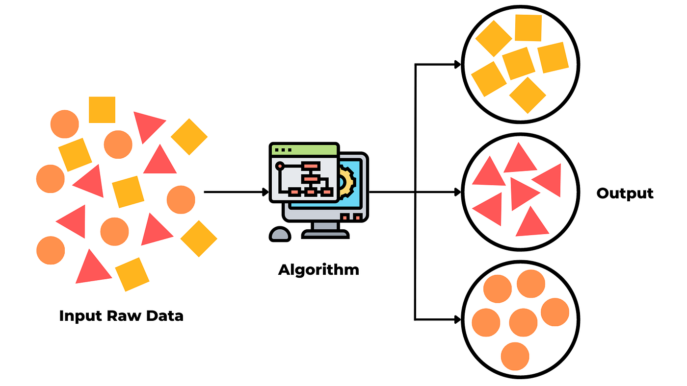
Unsupervised learning leverages data that contains no explicit labels or target values. Instead of being told “this input corresponds to that output,” the algorithm must uncover the underlying structure of the data on its own. In deep learning, this often takes the form of autoencoders, which compress and reconstruct inputs to learn compact feature representations, or generative models like GANs and VAEs, which learn to generate new samples matching the data distribution. Because it doesn’t need labels, unsupervised learning is ideal when manual annotation would be too slow or costly. You can feed in massive amounts of raw data to automatically discover clusters or latent variables, explore what’s hidden, and you can even speed up later supervised projects by feeding these automatically learned features into them, so you don’t have to label all your data by hand first.

Main Task Categories

• Clustering: Partition data into homogeneous groups (e.g., segment customers by purchasing behavior for targeted marketing).

  • Algorithms:

    • K-means: assign each point to the nearest centroid.
    • DBSCAN: group points by density, labeling low-density points as noise.

• Dimensionality Reduction: Find a compact representation of high-dimensional data (e.g., visualize gene-expression profiles in 2D to spot cell subtypes).

  • Algorithms:

    • PCA (Principal Component Analysis): linear projection that maximizes variance.
    • t-SNE or UMAP: nonlinear embeddings for visualization.

• Anomaly (Outlier) Detection: Identify rare or unusual observations (e.g., detect fraudulent transactions in financial records).

  • Algorithms:

    • Isolation Forest: builds random trees to isolate anomalies quickly.
    • One-Class SVM: learns a boundary around normal data.

• Representation Learning (Autoencoders, GANs): Learn compact, useful encodings of inputs (e.g., pretrain image encoders for downstream supervised tasks or generate realistic images).

  • Algorithms:

    • Autoencoder: compress and reconstruct inputs via a bottleneck layer.
    • Variational Autoencoder (VAE), Generative Adversarial Network (GAN).

Recommended Video - Unsupervised Learning Recommended Video - Latent Space

Reinforcement Learning

Reinforcement Learning (RL) is a machine-learning paradigm in which an algorithm learns to make a sequence of decisions by interacting with an environment and receiving rewards or penalties as feedback. Rather than learning from fixed examples (as in supervised learning) or mining unlabeled data (as in unsupervised learning), RL learns by trial and error, gradually improving its behavior to maximize cumulative reward.

Key concepts:

• Agent and Environment: The agent observes the current state $s$ of the environment, takes an action $a$, and the environment returns a new state $s^{'}$ plus a scalar reward $r$.

• Policy: A policy $\pi(a | s)$ defines the agent’s strategy—the probability of choosing action $a$ when in state $s$. Learning in RL means finding the policy that yields the highest total reward.

• Return and Discounting: The agent aims to maximize the return, often the sum of future rewards. In practice we use a discount factor $\gamma \in \left[0,1\right)$ so that

$$ \large G_t = r_{t+1} + \gamma,r_{t+2} + \gamma^2,r_{t+3} + \cdots $$

which balances immediate and long-term gains.

• Value Function: The value $V^{\pi}\left(s\right)$ is the expected return when starting in state $s$ and following policy $\pi$. It satisfies a recursive relation, but you can think of it simply as “how good is it to be in $s$ under $\pi$?”

Deep Reinforcement Learning

When states or actions are high-dimensional, such as images, audio or continuous controls, classical RL methods struggle. Deep RL addresses this by using a neural network to approximate:

• A value function $V_{\theta}(s)$ or an action-value function $Q_{\theta}​(s,a)$.

• A policy directly, as in Deep Policy Gradient methods.

Why Reinforcement Learning Matters

• Games: AlphaGo and AlphaZero learned superhuman strategies in Go and Chess purely by self-play.

• Robotics: Sim-to-real training lets robots learn manipulation or locomotion skills in simulation before transferring them to hardware.

• Autonomous Vehicles: Agents learn to make safe driving decisions by optimizing long-term safety and efficiency.

• Recommendation Systems: An RL agent can adapt suggestions to maximize long-term user engagement rather than immediate clicks.

Recommended Video - Reinforcement Learning

1.3 Foundations of Neural Networks

Rosenblatt's Perceptron

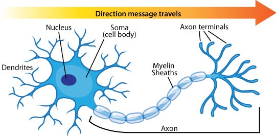
The perceptron, introduced by Frank Rosenblatt in 1958, is a simplified mathematical model of a biological neuron. In biology, a neuron consists of a cell body, dendrites (which receive signals) and an axon (which sends signals). Synapses connections between neurons can be excitatory (promoting firing) or inhibitory (suppressing firing). When enough excitatory input arrives, the neuron “fires”, passing its signal onward.

Core components of Roseblatt's perceptron:

• Inputs and Weights: Each input $x_{i}$​ is paired with a weight w_{i}. The weight determines how strongly that input influences the perceptron’s output. During learning, the perceptron adjusts these weights to correct its mistakes.

• Weighted Sum and Bias: The perceptron computes the weighted sum $z=\sum_{i=1}^{n} w_{i}x_{i} + b$, where $b$ is a bias term that shifts the activation threshold.

• Activation function: A step function converts the weighted sum $z$ into an output $y$:

$$ \large y = \begin{cases} 1, & \text{if } z \ge 0,\\ 0, & \text{if } z < 0. \end{cases} $$

This non-linearity allows the perceptron to make binary decisions.

• Learning Rule: After each example, the perceptron updates its weights based on the error $\left(\hat y - y \right)$:

$$ \large w_i \leftarrow w_i + \eta,\bigl(y - \hat{y}\bigr),x_i, \qquad b \leftarrow b + \eta,\bigl(y - \hat{y}\bigr) $$

This rule increases weights for inputs that should have fired and decreases them for inputs that fired incorrectly.

Multilayer Perceptrons

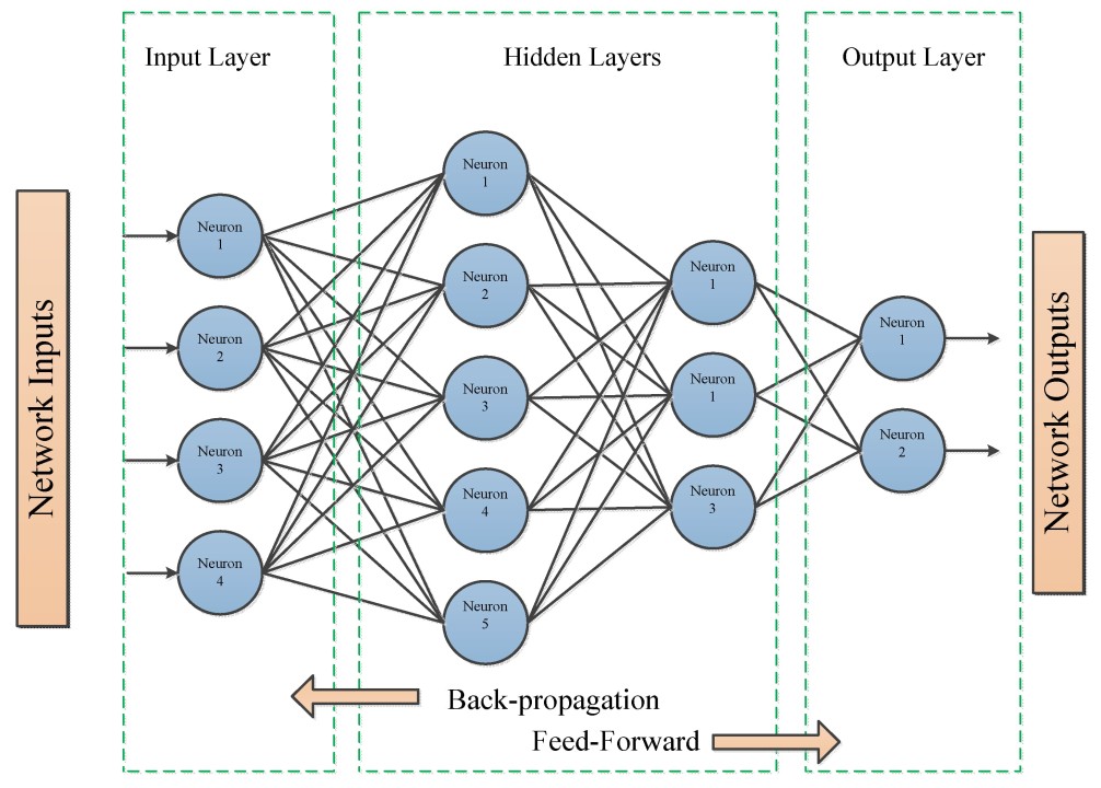
Multilayer Perceptrons (MLPs), or feedforward neural networks, extend the single‐layer perceptron by stacking several layers of weighted sums and nonlinear activations to approximate a target function $y = f^*(x).$ An MLP defines a parameterized mapping $y = f_{\theta}(x).$ where $\theta$ collects all weights and biases in the network. The network is built as a composition of $L$ layers:

$$ \large f_{\theta}(x) = f^{(L)}\bigl(a^{(L-1)}\bigr), \quad a^{(0)} = x. $$

and for each layer $\ell = 1, \dots, L$:

$$ \large z^{(\ell)} = W^{(\ell)}a^{(\ell-1)} + b^{(\ell)}, \qquad a^{(\ell)} = \sigma\bigl(z^{(\ell)}\bigr), $$

where

• $W^{\left (\ell \right)}$ and $b^{\left(\ell \right)}$ are the weight matrix and bias vector of layer $\ell$,
• $\sigma(\cdot)$ is a nonlinear activation (e.g. ReLU, sigmoid),
• $a^{(\ell)}$ is the layer’s output (sometimes called its activation).

The input layer $a^{(0)}$ simply holds the feature vector $x$, and the output layer $a^{(L)}$ produces the final prediction $f_{\theta}(x)$. During training, the parameters

$$ \large \theta = \lbrace W^{(\ell)},b^{(\ell)}\rbrace_{\ell=1}^L $$

are adjusted (via backpropagation and gradient descent) so that $f_{\theta}(x) \approx f^{*}(x)$ for all examples in the training set. The depth of the MLP is $L$, and its ability to model complex functions grows with more layers and neurons per layer.

1.4 Weight Initialization

Weight initialization plays a critical role in training deep neural networks, as it directly affects how signals and gradients flow through the model. A good initialization strategy can dramatically accelerate convergence and improve final performance by avoiding two notorious problems:

Vanishing Gradients: In backpropagation, gradients flow from the output layer back toward the input. If weights are initialized too small, or if activation functions squash their inputs into narrow ranges, these gradients shrink exponentially with each layer. As a result, updates become negligible, lower layers learn almost nothing, and training stalls or proceeds at a crawl.

This issue is especially acute with sigmoid or tanh activations, which saturate for large positive or negative inputs (their derivatives approach zero).

Exploding Gradients: At the other extreme, initializing weights too large can amplify gradients as they propagate backward. This can lead to unstable weight updates with excessively large parameter steps and may cause numerical overflow and divergence of the training process. Exploding gradients often surface in very deep models or recurrent architectures when initial weights have high variance.

To address these issues, weight initialization strategies are designed to ensure that gradients neither vanish nor explode. Some common approaches include:

• Xavier (Glorot) Initialization: This method initializes weights by drawing from a distribution with zero mean and variance inversely proportional to the number of input and output units. It is particularly effective for activation functions like sigmoid and tanh, as it helps maintain the variance of activations and gradients across layers.

• He Initialization: Specifically designed for ReLU (Rectified Linear Unit) activation functions, He initialization draws weights from a distribution with variance proportional to the number of input units. This approach helps mitigate the issue of vanishing gradients in networks using ReLU activations.