Exploration

Jump to bottom

kosh edited this page Feb 28, 2022 · 12 revisions

Utils

`embedding`

Generate a time series using the embedding dimension D and the time lag L.
Embedding uses the delayed coordinate system shown below.

$\mathbf{x}(t)=(x(t), x(t+T), ..., x(t+(D-1)T))$

from hundun import embedding
# ok -> from hundun.exploration import embedding

Parameters

u_seq
T
D

Returns

e_seq

Example

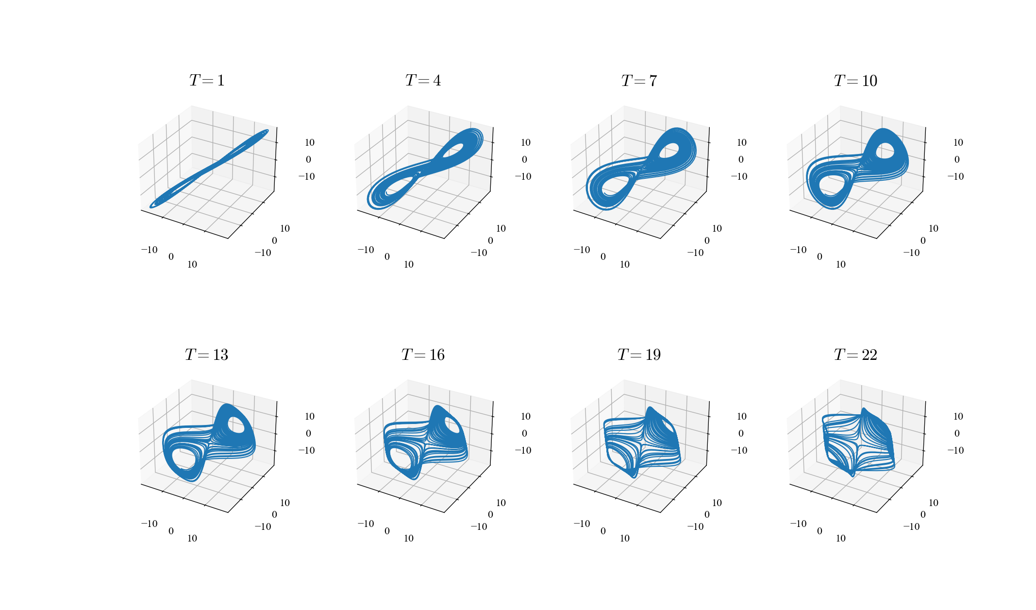
An example is shown using x in the three-dimensional time series (x, y, z) obtained from the Lorenz equation.
Fix it at D=3 and draw while shifting T by 3.

from hundun import Drawing
from hundun.equations import Lorenz
from hundun.exploration import embedding

x_seq = Lorenz.get_u_seq(5000)[:, 0]

d = Drawing(2, v:=4, three=True)
for i in range(8):
    s, T = divmod(i, v), i*3+1
    e_seq = embedding(x_seq, T, 3)  # <- here
    d[s].set_title(f'$T={T}$')
    d[s].plot(e_seq[:, 0], e_seq[:, 1], e_seq[:, 2])
d.show()

img:embedding_T

`acf`

Calculate the autocorrelation function from the time series data.

The autocovariance function $gamma$ is calculated from the following formula.

$\gamma(\tau)=\frac{1}{N-\tau}\sum_{t=0}^{N-1-\tau}( x(t) - \bar{x} )( x(t+\tau) - \bar{x} )$

The autocorrelation function $rho$ is estimated as follows.

$\rho(\tau)=\frac{\gamma(\tau)}{\gamma(0)}$

from hundun.exploration import acf

Parameters

u_seq
tau

Returns

rho_seq_list: List[numpy.ndarray]

`bartlett`

dev

Calculate the time series with Barrett's formula.

Calculate $B$ using the standard deviation quantile $z$ in $alpha$ .

$B=z_aSE(seq_h)$

$SE(seq_1)=\frac{1}{\sqrt{N}}$

$SE(seq_h)=\sqrt{\frac{1+2\sum_{i=1}^{h-1}{r_i^2}}{N}}$

from hundun.exploration import bartlett

Parameters

seq
alpha=0.95

Returns

B: numpy.ndarray

`mutual_info`

Calculate mutual information $I$ by creating a histogram. Calculate from the following formula using information entropy.

$I({x(t)} \ ; {x(t+\tau)})=H({x(t)} )+H({x(t+\tau)} ) - H({x(t)} , {x(t+\tau)} )$

from hundun.exploration import bartlett

Parameters

u_seq
tau

Returns

mi_seq: numpy.ndarray

Home / Repo / PyPI