Lyapunov exponents

Calculate the Lyapunov exponents (Lyapunov spectrum).

calc_les

Compute the Lyapunov spectrum for a given Differential or Difference. (That is, system must be a DynamicalSystems)

Different calculation methods are used for Differential and Difference equation. In Differential equation, the calculation method differs depending on the presence or absence of the Jacobian Matrix.

See the example for usage.

Params

• system
• **options

Returns

• les_seq: numpy.ndarray
• les: Tuple(float)

Examples

• Example - Difference
  • Logistic map (1)
  • Logistic map (2)
  • Henon map (1)
  • Henon map (2)
• Example - Differential
  • Lorenz equation

Difference

Jacobin is always required because it is calculated on the QR base. (In the case of 1-dim, a different method is used instead of QR-based to speed up the calculation.)

Logistic map (1)

Calculate the Lyapunov exponent at .

les_seq shows the calculation process and can be confirmed whether it has converged.

import math

from hundun import calc_les
from hundun.equations import Logistic
from hundun.utils import Drawing


les_seq, le = calc_les(Logistic, N=1000, a=4)
print(le)

d = Drawing()
d[0,0].plot(les_seq)
d[0,0].axhline(math.log(2), color='red')
d[0,0].set_xlim(0, 999)
d[0,0].set_ylim(0.6, 0.8)
d.show()

[0.6929778]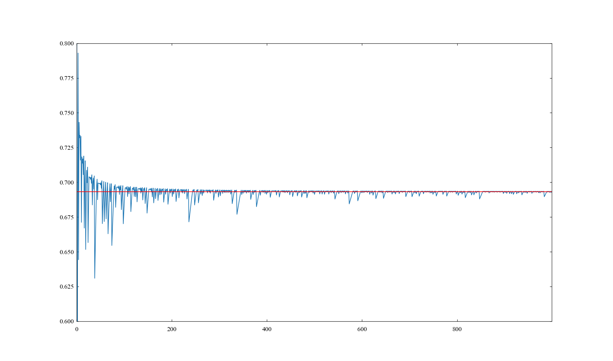

Logistic map (2)

As an example, calculate the LE for parameter of Logistic map.

import math

from hundun import calc_les
from hundun.equations import Logistic
from hundun.utils import Drawing


a_list, le_list = [], []
for i in range(L:=400+1):
    a = i*0.01
    _, le = calc_les(Logistic, N=500, a=a)
    le_list.append(le)
    a_list.append(a)

d = Drawing()
d[0,0].plot(a_list, le_list)

options = {'linewidth':0.5, 'linestyle':'dashed'}
d[0,0].axhline(0, color='black', **options)
d[0,0].axhline(math.log(2), color='red', label=r"$\ln2$", **options)

d[0,0].legend(loc='lower right')
d[0,0].set_axis_label('a', r'\lambda')
d[0,0].set_ylim(-4, 1)
d[0,0].set_xlim(0, 4)
d.show()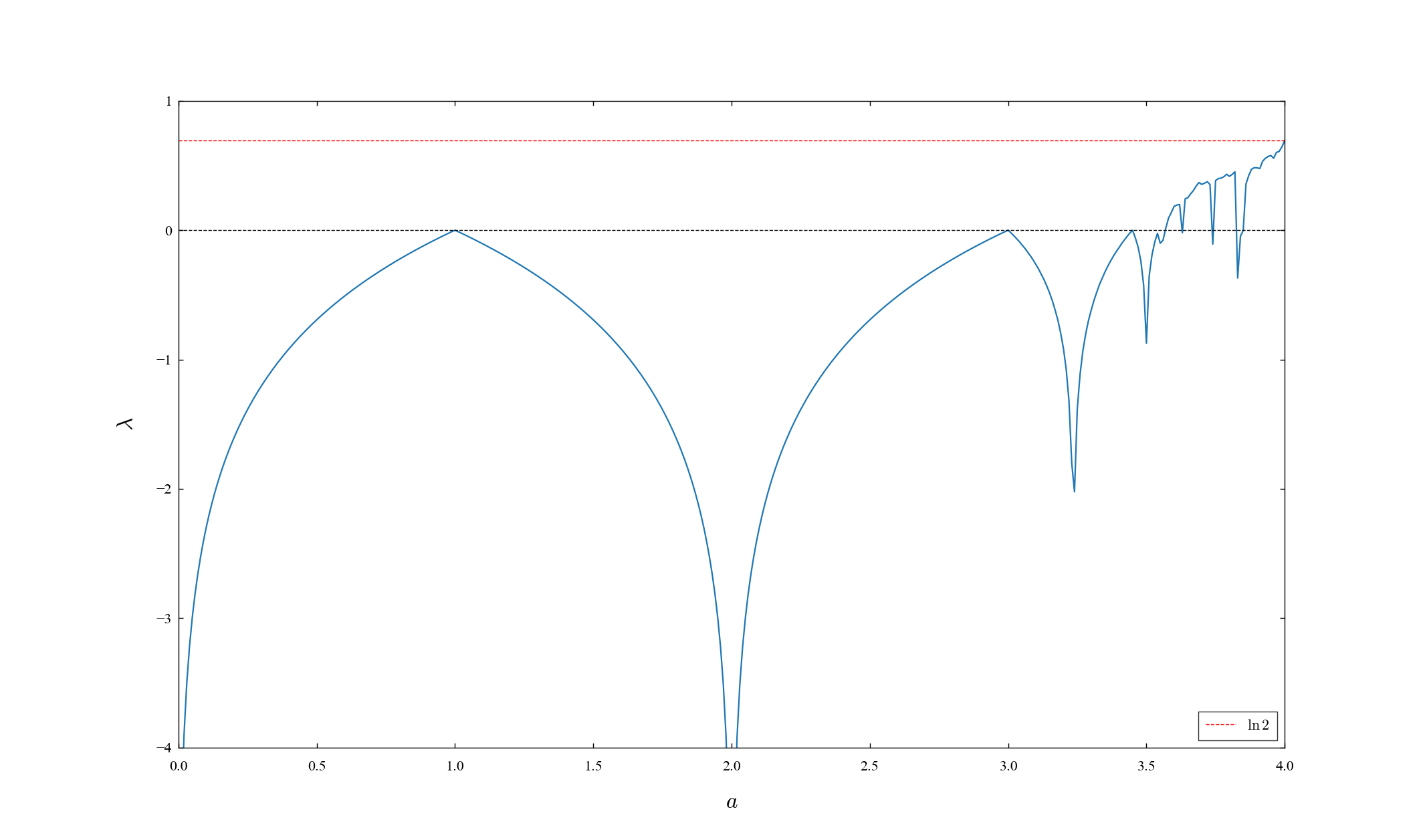

Henon map (1)

Calculation of Lyapunov spectrum at .

from hundun import calc_les, Drawing
from hundun.equations.henon import Henon


les_seq, les = calc_les(Henon, a=1.4, b=0.3)
print(les)

d = Drawing()
for i in range(2):
    d[0,0].plot(les_seq[:, i], zorder=10,
                label=rf'$\lambda_{i+1}$')
    d[0,0].axhline(les[i], zorder=1,
                   linestyle='dashed', color='black', linewidth=0.5)
d.legend()
d.show()

[ 0.41653372 -1.62050652]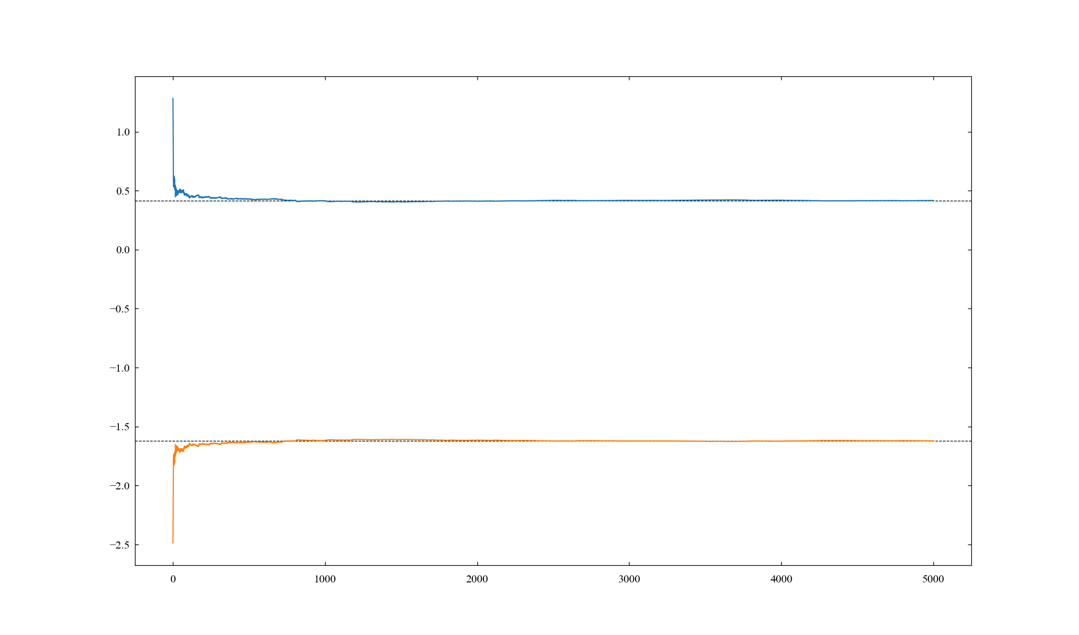

Henon map (2)

As an example, search for parameters of Henon. It is possible to estimate the range in which the LEs is positive.

from itertools import product

from hundun import Drawing, calc_les
from hundun.equations.henon import Henon
from matplotlib.colors import Normalize
import numpy as np


N_a, N_b = 50, 50
a_list = np.linspace(0, 2.1, N_a)
b_list = np.linspace(0, 1.1, N_b)

les_list = []
for a, b in product(a_list, b_list):
    for _ in range(10):
        try:
            _, les = calc_les(Henon, b=b, a=a)
            les_list.append(les)
            break
        except ValueError:
            pass
    else:
        les_list.append((None, None))
les = np.array(les_list).reshape(N_b, N_a, 2)

d=Drawing(1, 2)
for i in range(2):
    le = les[:,:,i]
    sf = d[0,i].contourf(*np.meshgrid(a_list, b_list), le, cmap='jet',
                         norm=Normalize(vmin=-2, vmax=1))
    cb = d.fig.colorbar(sf, ax=d[0,i], orientation='horizontal')
    d[0,i].set_axis_label('a', 'b')
    d[0,i].set_title(fr'$\lambda_{i+1}$')
d.show()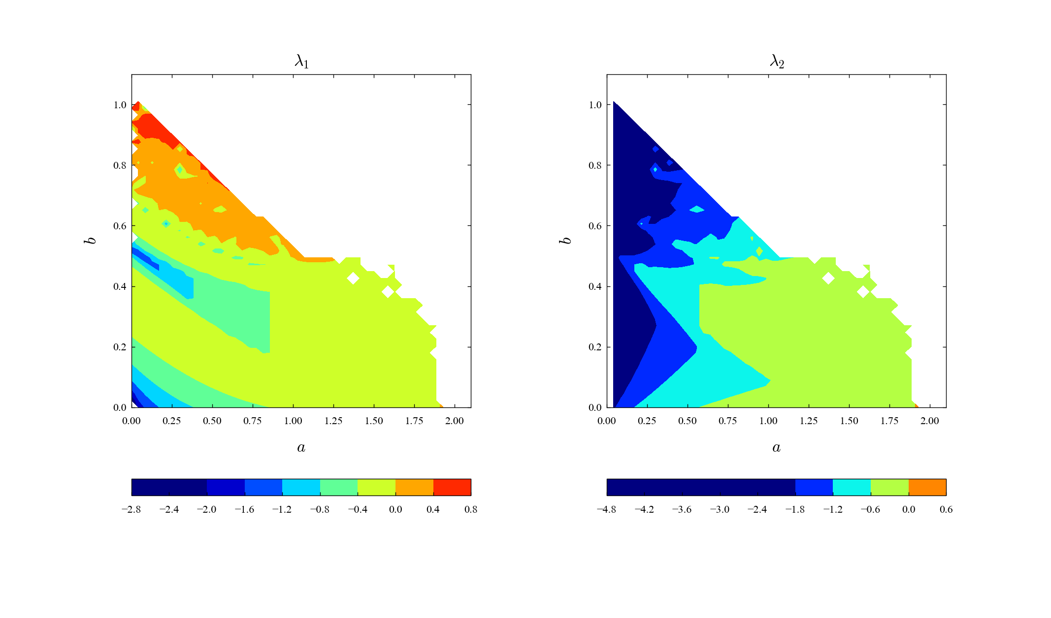

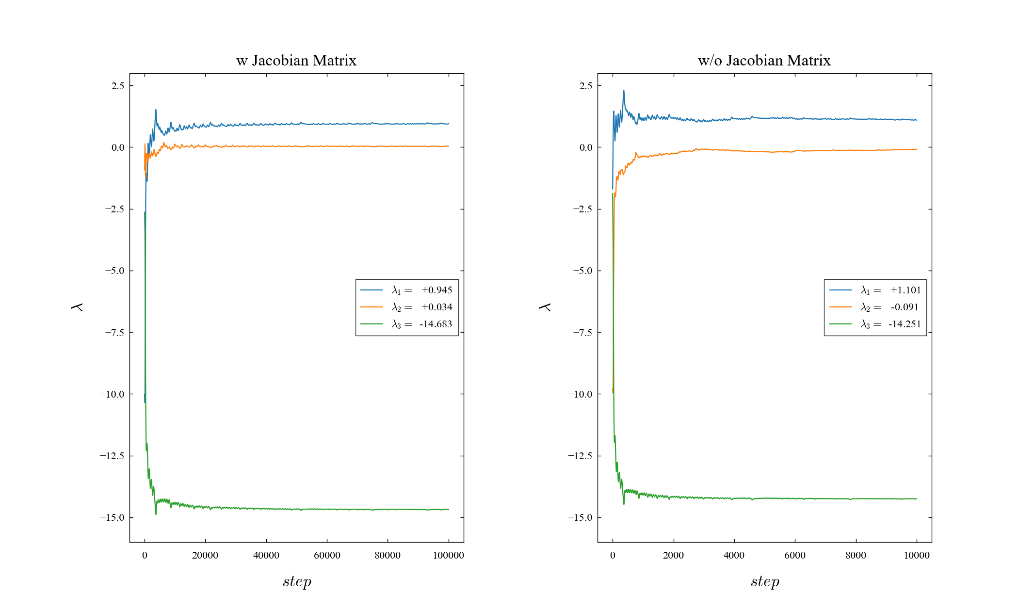
Differential

Jacobian Matrix is not mandatory.

If Jacobian Matrix does not exist, LEs will be calculated based on the orbit.

Let's check the implementation of Lorenz. The Jacobian Matrix is implemented as follows.

class Lorenz(Differential):

    def parameter(self, s=10, r=28, b=8/3):
        self.s, self.r, self.b = s, r, b
        self.dim = 3

    def equation(self, t, u):
        s, r, b = self.s, self.r, self.b

        x, y, z = u

        x_dot = s*(y - x)
        y_dot = r*x - y - x*z
        z_dot = x*y - b*z

        return x_dot, y_dot, z_dot

    def jacobian(self):
        s, r, b = self.s, self.r, self.b
        x, y, z = self.u

        j = [[-s, s, 0],
             [r-z, -1, -x],
             [y, x, -b]]

        return j

Lorenz equation

The left side of the graph is when QR decomposition is used, and the right side is when calculated from the orbit. The absence of Jacobian Matrix means that the return value is None or does not exist in the first place.

from hundun import calc_les, Drawing
from hundun.equations import Lorenz


class Lorenz_No_Jacobian(Lorenz):
    def jacobian(self):
        return None


u0 = Lorenz.on_attractor().u

d = Drawing(1, 2)
for j, system in enumerate([Lorenz, Lorenz_No_Jacobian]):
    les_seq, les = calc_les(system, u0=u0)
    print(les)
    for i, le in enumerate(les):
        p, = d[0, j].plot(les_seq[:, i],
                          label=fr'$\lambda_{i+1}=$ {le:>+8.3f}')

    d[0,j].legend(loc='center right')
    d[0,j].set_axis_label('step', r'\lambda')
    d[0,j].set_ylim(-16, 3)
    d[0,j].set_title(f"{'w' if j==0 else 'w/o'} Jacobian Matrix")
d.show()

[  0.94490089   0.03358318 -14.68297111]
[  1.10108133  -0.09147609 -14.25104879]