3.2. Hands On: Distributed Sensorization

The sensorization example represents a typical industrial use case where it is needed to monitor a certain process. To abstract this process, we will simulate and integrate a sensor with a database, at the end we will see the sensor data in a common dashboard. For that, each Raspberry Pi simulates a sensor that produces values with a certain range and offset, these values are processed by a method (e.g. moving average) and then, both original value and his moving average are published in an MQTT Broker. Another machine is responsible for the interface between the MQTT Broker and the Time Series Database (InfluxDB), where is stored all the data from the process. This interface is needed to subscribe to the values from the MQTT Broker and then write these values in the InfluxDB, using a remote client. Based in that, the process that we want to develop is the following:
Sensor Simulator -> Moving Average -> MQTT Publisher -> MQTT Subscriber -> Influx DB
For that, we build a mini Cyber-Physical System (CPS), where the Sensor Simulator, the Moving Average, and the MQTT Publisher function blocks are running in a Raspberry Pi and the MQTT Subscriber and the Influx DB Writer are running in your PC.

This mini CPS has used some extra resources: 1) MQTT Broker, that runs in your Raspberry Pi, and 2) InfluxDB and Grafana Server (graphics visualization, alarms), that are running in another Raspberry Pi.
To build this solution we need to use 5 different function blocks, each function is composed by 2 files (XML and Python), wherein the XML file is defined the interface (input/output events, input/output variables) and in the Python file are coded the function block functionalities.
| Function Block | Resources | Description |
|---|---|---|
| Sensor Simulator | [XML] [Python] | Simulates the sensor values according one offset |
| Moving Average | [XML] [Python] | Calculates the average of the last N values |
| MQTT Publisher | [XML] [Python] | Publishes a message with 2 values in the MQTT Broker |
| MQTT Subscriber | [XML] [Python] | Subscribes a message with 2 values from the MQTT Broker |
| Influx DB Writer | [XML] [Python] | Writes 2 values in a time series database |
You can also download the 4DIAC configuration [ZIP], to import in the 4DIAC-IDE using the option File->Import->Existing Projects into Workspace, and selecting the root path to the 4DIAC configuration. This way, you acelerate the development process, skiping some of the steps of the following tutorial.
In the machine(s) that execute the DINASORE runtime environment, you must guaranty that the FBs have their PIP dependencies installed. For the tutorial FBs, the PIP dependencies are [influxdb] [paho-mqtt], use the command pip install "package" to install it.
-
Execute the DINASORE project in your computer, commands here;
-
Copy the .fbt files from the function blocks DINASORE folder to a new 4DIAC-IDE function blocks folder (.../4diac-ide/typelibrary/(new_folder));
-
Run the 4DIAC-IDE executable (.../4diac-ide/4diac-ide);
-
Create a new system using File->New->New System, call the new system e.g. SensHandsOn and click Finish;
-
Open the System Configuration tab and drag and drop 2 FORTE_PC devices and 1 Ethernet segment, from the Palette;

-
Change the IP addresses and component names according to the machines that you have in the network;
-
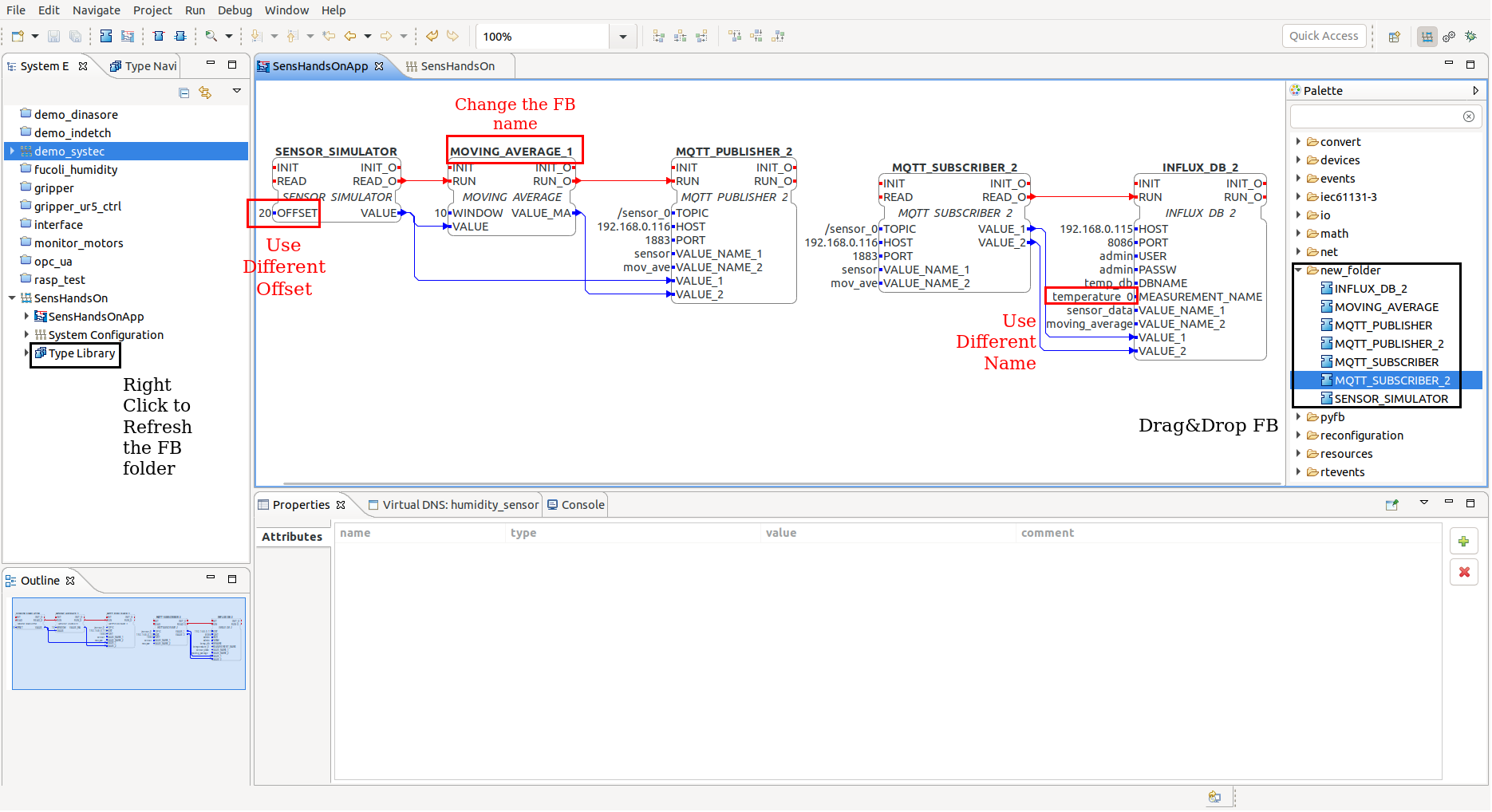
Double click on the 'SensHandsOnApp' (FB Configuration) view using the left bar;
-
Drag&Drop the function blocks from a new folder in the right Palette;
-
Connect each event and variable, and specify the hardcoded value for some variables (e.g. IP address, port, DB name);
-
Each one must specify 1) a different offset (e.g. multiples of 10) for the sensor simulator function block and 2) a different measurement name (different index) (InfluxDB FB), for better visualization of all the sensors in the Grafana dashboard;
-
Map each function block to a network component (e.g. right click on function block them select Map to...->FORTE_PC->RASP_COMP);

-
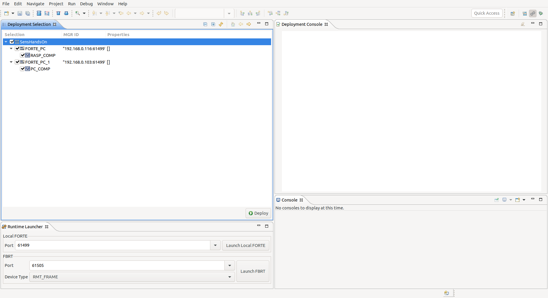
Change to the Deploy View (right corner icon or Window->Perspective->Open Perspective->Deployment);
-
Select your configuration and click 'Deploy' to upload the configuration to the Smart Components;
- To monitor the system, change to the previous view, then right-click on the project folder and select Monitor System. Now you can select which variables you want to monitor, for that right-click inside the variable and select Watch;

-
To stop the monitoring process, right-click in the project folder and select Remove Watches and unselect Monitor System;
-
If you want to reset each component, right-click in his name in the left bar and select Delete all Resources;
-
Alternatively, you are able to visualize the data from the sensors using the Grafana Dashboard. Open your browser and type the URL: 192.168.0.115:3000 (user:admin, password:admin);

-
In the Grafana page you are able to plot data columns from the InfluxDB, add alarms to the dashboard and use many other plugins;
-
The URL 192.168.0.115:8083 allow you to manage the administration options of the InfluxDB, like search queries or add/delete databases;

- Finally, to check the data structure or monitor the process using OPC-UA, you can use the Prosys client, connecting to the component IP address at port 4840.
