Supervised Learning
"Remember that supervise learning is used when ever we want to predict a certain outcome from a given input, and we have examples of inputs/output pairs. We build a machine learning model from these input/output pairs, which comprise a training set. Our goal is to make accurate predictions for new, never before seen data. Supervise learning often requires human effort to pull the training set, but afterwards automates and often speeds up an otherwise laborious or infeasible task." Quoted from Introduction to machine learning in Python
There are two different types of problem spaces that machine learning problems solve:
Classification is the grouping that we place a result in. Formally this is referred to as a class label. Classification can either be a binary classification which behaves simlarly to yes/no questions. The other is a multiclass classification which can group into multiple classes (like the iris species from the introduction).
The goal for regression is to predict a continuous number (non-discrete). An example of this is shown in the introduction exercise which uses features from music to determine how many likes/listens it will have rather than a genre of music (this would be a classification).
And supervise learning we want to build a model that can make accurate predictions on new unseen data. If the model is able to do this we say it is able to generalise from the training set for test set. Sometimes our predictions can be compromised by the quality of our data/models.
In statistics, a fit refers to how well you approximate a target function.
This is good terminology to use in machine learning, because supervised machine learning algorithms seek to approximate the unknown underlying mapping function for the output variables given the input variables.
Statistics often describe the goodness of fit which refers to measures used to estimate how well the approximation of the function matches the target function.
Some of these methods are useful in machine learning (e.g. calculating the residual errors), but some of these techniques assume we know the form of the target function we are approximating, which is not the case in machine learning.
Overfitting happens when a model learns the detail and noise in the training data to the extent that it negatively impacts the performance of the model on new data. This means that the noise or random fluctuations in the training data is picked up and learned as concepts by the model. The problem is that these concepts do not apply to new data and negatively impact the models ability to generalize.
An underfit machine learning model is not a suitable model and will be obvious as it will have poor performance on the training data.
Ideally, you want to select a model at the sweet spot between underfitting and overfitting.
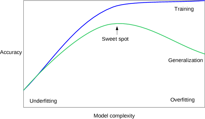
This is the goal, but is very difficult to do in practice.
To understand this goal, we can look at the performance of a machine learning algorithm over time as it is learning a training data. We can plot both the skill on the training data and the skill on a test dataset we have held back from the training process.
Over time, as the algorithm learns, the error for the model on the training data goes down and so does the error on the test dataset. If we train for too long, the performance on the training dataset may continue to decrease because the model is overfitting and learning the irrelevant detail and noise in the training dataset. At the same time the error for the test set starts to rise again as the model’s ability to generalize decreases.
The sweet spot is the point just before the error on the test dataset starts to increase where the model has good skill on both the training dataset and the unseen test dataset.
There are two additional techniques you can use to help find the sweet spot in practice: resampling methods and a validation dataset.
Overfitting: Good performance on the training data, poor generliazation to other data. Underfitting: Poor performance on the training data and poor generalization to other data
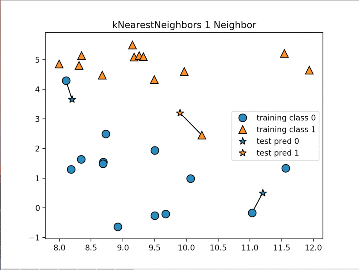
The K-Nearest Neighbors (k-NN) algorithm is considered one of the simplest machine learning algorithm. Once the training and test datasets have been stored the algorithm makes a prediction for a new data point, the algorithm finds the closest data points in the training dataset - it's "nearest neighbors"

Example of k-NN classification. The test sample (green circle) should be classified either to the first class of blue squares or to the second class of red triangles. If k = 3 (solid line circle) it is assigned to the second class because there are 2 triangles and only 1 square inside the inner circle. If k = 5 (dashed line circle) it is assigned to the first class (3 squares vs. 2 triangles inside the outer circle).
There are two primary properties that influence the KNeighbors Algorithm. The first is changing the number of neighbors we are measuring against. As we increase the number of neighbors we decrease the complexity of our model. The image below shows how changing the number of neighbors affects the decision of our algorithm. The other property is the way we measure the distance between the various data points. The most commonly used method is the euclidean distance which is the ordinary straight line distance between the two data points.
The next image displays the decision boundaries for the various numbers of neighbors:
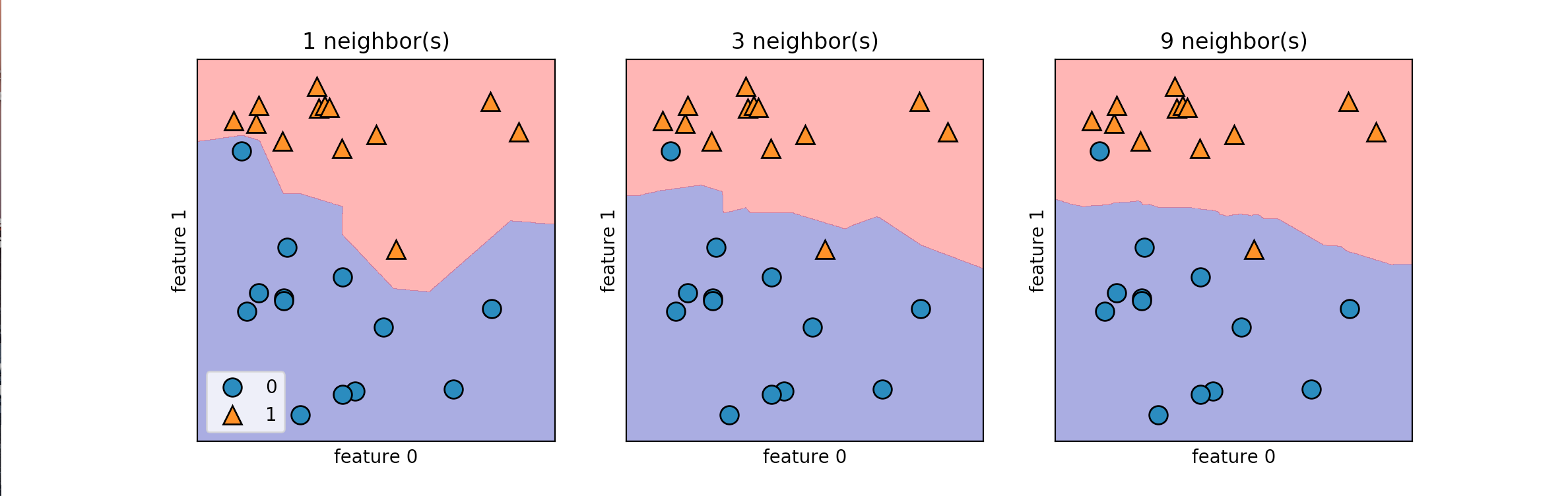
As the number of neighbors increases our model is simplified resulting in smoother boundaries between the two classifications. For an interactive model of KNearestNeighbors check out this site
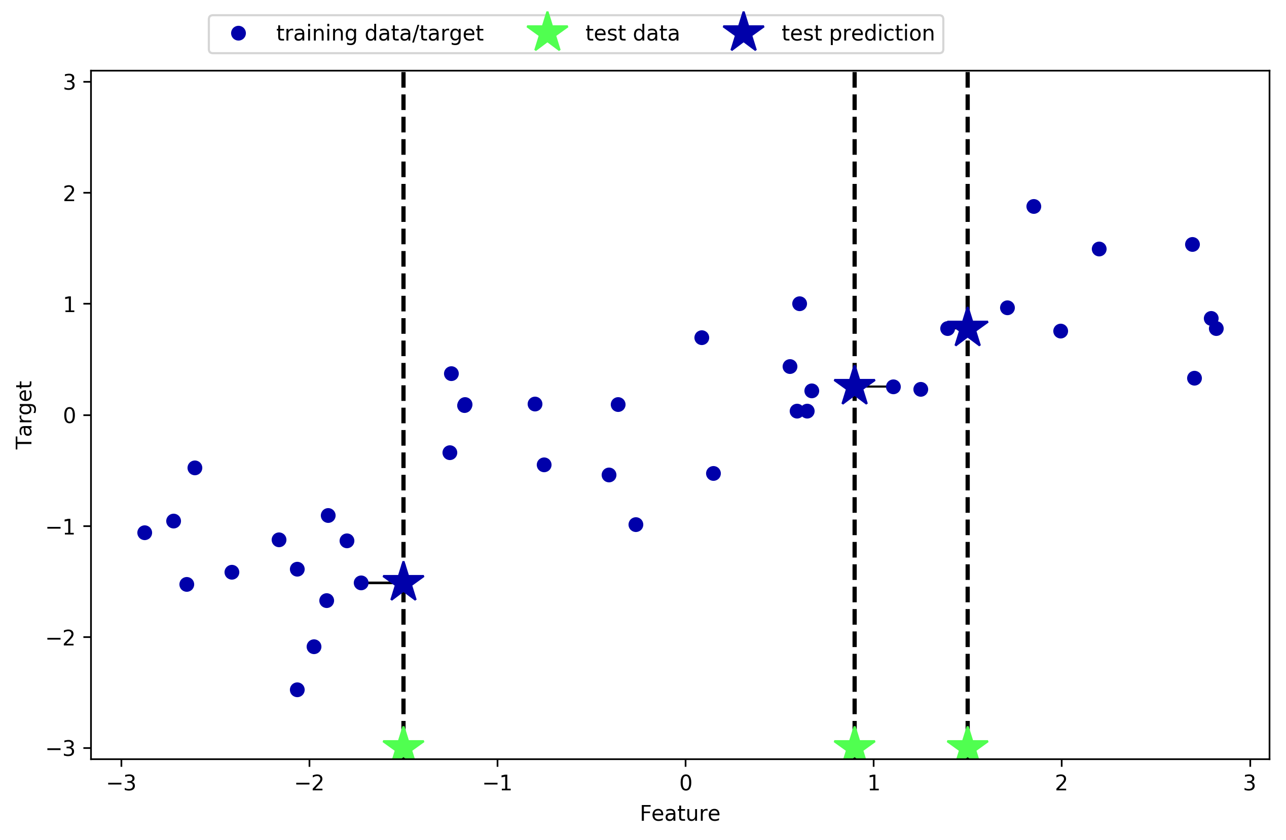
This same process can be run on the KNeighbors Regression which behaves the same as previosuly but for non-discrete results.
One of the strengths of k-NN is that the model is very easy to understand and often gives reasonable performance without a lot of adjustments. Using this algorithm is a good baseline method to try before considering more advanced techniques. Building the nearest neighbors model is usually very fast, but when your training set is very large predictions can be slow. This approach often does not perform well on datasets with many features (hundreds or more), and it does particularly badly with datasets where most features are 0 most of the time (sparse datasets).
While the nearest k-neighbors algorithm is easy to understand, it is not often used in practice, due to prediction being slow and its inability to handle many features. The method we discuss next has neither of these drawbacks.
Linear models are a class of models used in wide practise. They make predictions using linear function of the input features.
The term linear model implies that the model is specified as a linear combination of features. Based on training data, the learning process computes one weight for each feature to form a model that can predict or estimate the target value. For example, if your target is the amount of insurance a customer will purchase and your variables are age and income, a simple linear model would be the following:
Estimated target = 0.2 + 5.age + 0.0003.income
The way we perform predictions using this model is by assigning a weighting to each feature and an overall offset. The general prediction formula for linear model for a single feature is as follows:
y = w[0] . x[0] + b
y: prediction
w: weighting
x: feature
b: offset
Linear regression is the simplest linear method for regression. Linear regression finds the parameters w and b that minimize the mean squared error between predictions and the true regression targets. The mean squared error is the sum of the squared differences between the prediction and the true values, divided by the number of samples. The w parameter is the "slope" parameter and is the weighting we apply to a particular feature. The b parameter is the intercept which is the offset when the feature is 0.
Ridge regression is also a linear model for regression, so the formula is the same as the one used for ordinary least squares. In ridge regression, though , the coefficients (w) are chosen not only so that they predict well on the training data but have one additional constraint. The magnitude of the coefficient must be as small as possible; in other words, all entries of w should be as close to zero. This means all features should have as little effect on the outcome as possible while still predicting well. This constraint is called regularization. Regularization means explicitly restricting a model to avoid overfitting.
An alternative to Ridge for regularising liner regression is Lasso. As with ridge regression, using the lasso also restricts coefficients to be close to zero, but in a slightly different way. This means that some features are entirely ignored by the model. This can be seen as an automatic selection. Having some coefficients being zero can often make a model easier to interpret and can reveal the most important features of your model.
VISUALIZATION OF DIFFERENT ALPHA VALUES
Linear models can be used for classification
In this case the value we get from a linear model algorithm (remember it behaves similar to a straight line equation) gets classified to one group if >0 and the other if <0
EXAMPLE OF LINEAR MODEL
These classification models have a parameter related to the strength of regularization 'C' (the amount we try to minimize the effect of individual features). The higher this value, the less regularization.
Decision trees are widely used models for classification and regression tasks. Essentially they learn a hierarchy of it/else questions, leading to a decision
DECISION TREE EXAMPLE
DECISION TREE PROGRESSION