5. Characterize the Helium Probe of a Vessel
This chapter shall help to correctly characterize the superconducting liquid helium probe of a vessel or cryostat. At first, an introduction and the background are explained regarding how the probe works and which problems occur that must be handled. This is followed by an in-depth explanation of how to set up the probe and how to find the best operating parameters. First, an introduction regarding the operating current (also called optimum current in the following) is given with an added cooking recipe as a short form of this, followed by an explanation regarding the minimum and maximum resistances of the probe.
A superconducting wire with a critical temperature above 4.2 K embedded in a matrix with relatively high resistance (for example NbTi with T_C≈10 K in CuNi matrix) can be used as sensor for the liquid helium probe. The measurement principle relies on the idea that when the wire is introduced to a vessel or cryostat filled with liquid helium, the section below the liquid helium level becomes superconducting while the part above maintains its electrical resistance. This means, by measuring the total electrical resistance of the wire, the filling level of the vessel or cryostat can be determined.
The measurement principle itself is based on applying a current to the superconducting wire and measuring the voltage drop across it (see fig. 15). Normally, for a 4-point measurement two wires would be used for applying the current and two additional ones for measuring the voltage drop (in the diagram Circuit option 1). Based on the assumption of a negligible resistance of the supply wires a 3-point measurement is also possible (in the diagram Circuit option 2).
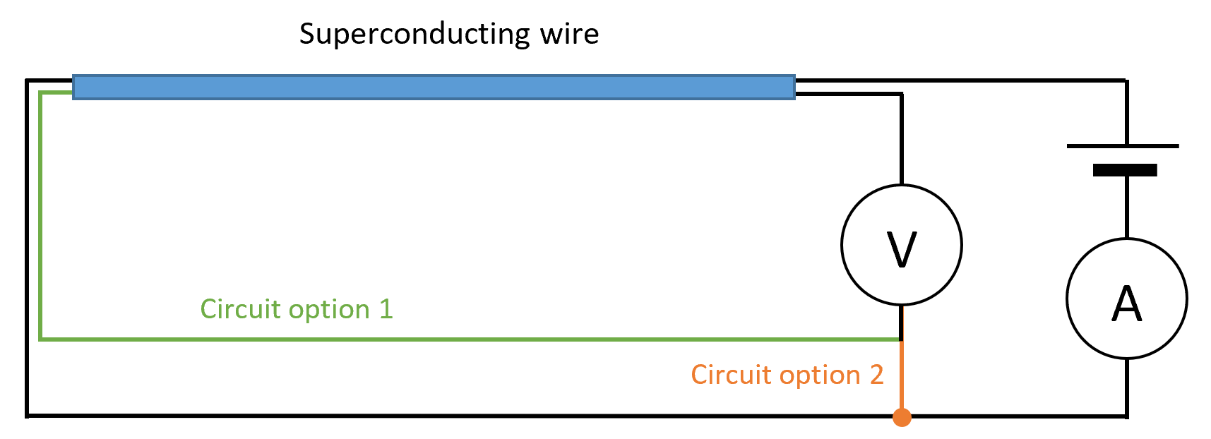
Figure 15: General principle of the resistance measurement of a superconducting helium probe with two options of choosing the supply wires.
However, in reality a certain section of the wire just above the liquid level is typically also in the superconducting state due to thermal conduction along the wire and the temperature profile in the vessel or cryostat which complicates reliable measurements. Different configurations exist regarding the embedding of the wire and the operation to solve this problem and to get reliable measurement results. Regarding the embedding, for example a not-superconducting wire can be wound around the superconducting wire to heat it externally and thus to compensate for the problematic cooling in the gaseous phase [1]. Another setup uses the measurement current to propagate the not superconducting zone along the superconducting wire until it stops at the liquid-vapor interface. Regarding the operation, there also exists another approach for this setup: Instead of heating only to the interface, the whole wire can be heated including the part in the liquid by choosing a sufficient high current. Afterwards, the liquid helium cools the part of the wire in the liquid and lets return it to the superconducting state while the remaining length stays in the normal conducting state. The desired voltage drop is measured then, using a lower current. These two methods of operation are also called One-Current and Two-Current Approach.
Here, following the argumentation of [2], the preferred approach consists in the direct heating of the superconducting wire with a current because of high boil-off rates of the other configurations. This configuration, in turn, should be operated using the one-current approach to reduce the heat in-leak and the measurement time [2]. However, the helium level meter is also capable of using the two-current approach. This can be necessary for probes without a resistance soldered to the superconducting wire where high currents are necessary to heat the wire. Furthermore, a slightly higher current at the beginning can speed up the measurement in the One-Current Approach.
As written, the One-Current method consists in heating the wire with a sufficiently high current to propagate the normal conducting phase towards the liquid-vapor interface. The challenge in doing so consists in choosing the optimum current to quench the whole part in the gaseous phase without propagating into the liquid – independent of liquid level and boil-off rate. For some current values the liquid-vapor interface will coincide with the threshold between superconducting and normal conducting state due to the different heat transfer in the gaseous and the liquid phase. Considering amongst others the convection in the vapor phase which implies a varying heat transfer coefficient along the wire and further effects by thermal contacts and the outer protective tube, it becomes clear that for a specific range of currents the normal conducting state will stop its propagation somewhere in the gas phase above the liquid. The same applies to the liquid phase. Finally, above a certain current value the whole wire is turned into the normal conducting state. Above this value the resistance of the wire is constant at maximum value. The explained processes and the corresponding current ranges can be seen in figure 16 where schematically the resistance of a superconducting helium probe is plotted over time for different currents from I_Range1 to I_Range5.
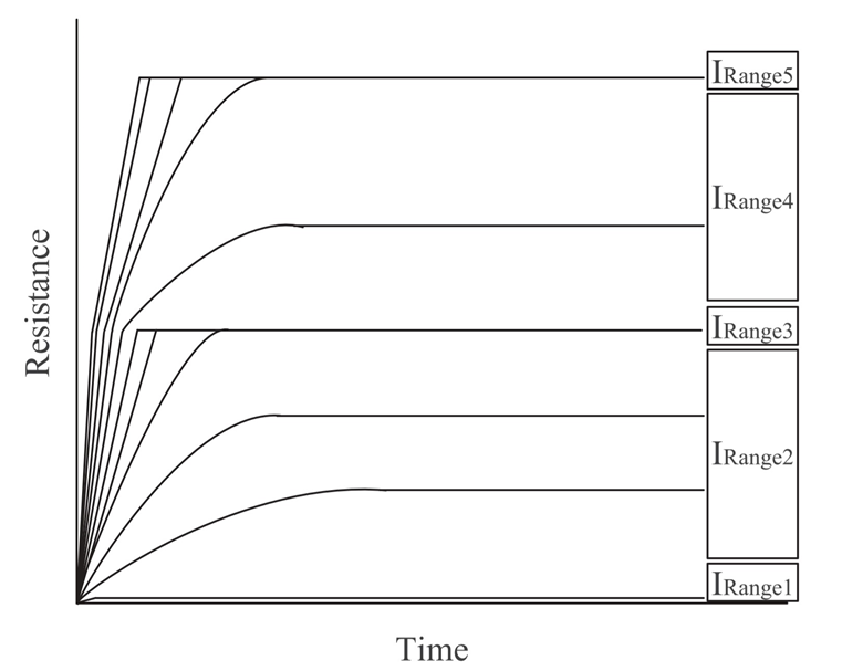
Figure 16: Expected resistance versus time graph – optimum current analysis from [2]. I_Ranges are explained in the text. I_Range3 corresponds to the optimum current range which turns the sensor part above the vapor liquid interface into the normal conducting state while the lower part in the liquid helium remains superconducting. A current in this range must be used to get reliable measuring results for determining the liquid helium level.
The current range I_Range1 coresponds to a completely superconducting probe with a resistance of near zero. This occurs when the current is too small to turn any part of the wire into the normal conducting state. When the current is increased (I_Range2), some length of the wire can be turned into the normal conducting state, but the normal conducting section does not get to the vapor liquid interface. By further increasing the current (I_Range3), the normal conducting zone of the wire reaches the interface. The current range leading to this constant resistance reading corresponds to the optimum current range I_Range3 because this is the searched value. At significantly larger currents corresponding to I_Range4 the normal conducting zone penetrates into the liquid. When the current is so high that the whole wire is turned into the normal conducting state the maximum resistance of the probe will be measured. The related current range is I_Range5. The change of slope at the steady state resistance of I_Range3 results from a better heat transfer of the liquid which slows the propagation of the normal zone. Furthermore, it can be seen that a higher heating power results in a faster propagation of the normal conducting zone.
The circuit diagram of the superconducting helium probe is shown in figure 17. In our case only three supply wires are used to reduce the heat in-leak. An external heater should be used at the current leading line at the top to have a starting point for the propagation of the normal conducting zone even when the whole wire is in the superconducting state. The external heater can for example be an SMD resistor which is well integrable due to its small size. Finally, the three supply wires must be soldered to the contacts of the LEMO plug in accordance with figure 3.
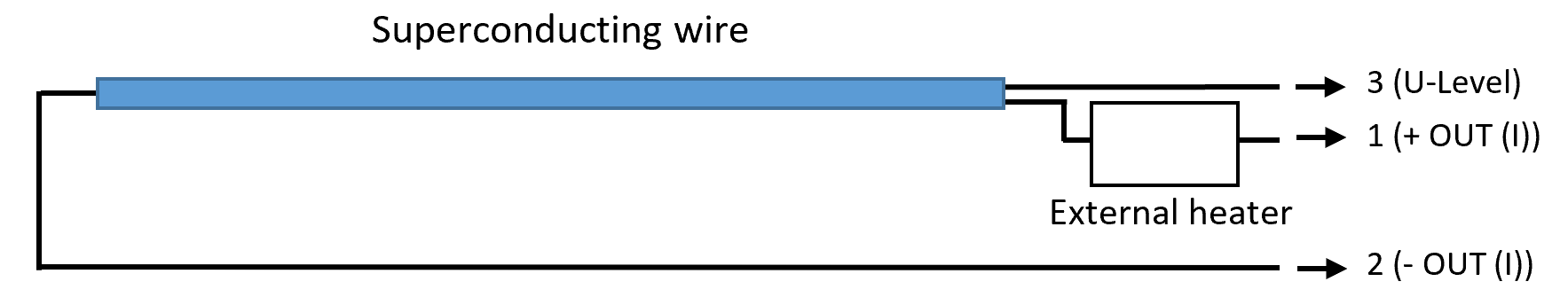
Figure 17: Circuit diagram of the resistance measurement of a superconducting helium probe for the use with the HZB level meter and assignment to the pins.
At the end of this subchapter a cooking recipe is added which summarizes all steps to find the optimum current, which is explained in more detail in the following.
Many parameters affect the optimum current which has to be applied to measure the resistance of the probes’ length inside the gaseous phase and to determine the liquid helium level. This e.g. includes the material of the superconducting wire, the diameter, the length, the convection in the gaseous phase, the boil-off rate and the thermal coupling to the housing tube. There are two ways of finding the optimum current: Calculating or determining experimentally.
A mathematical model has been established by Kunniyoor et al. [3] which was already validated experimentally where the computational results showed good agreement with the experimental data [2].
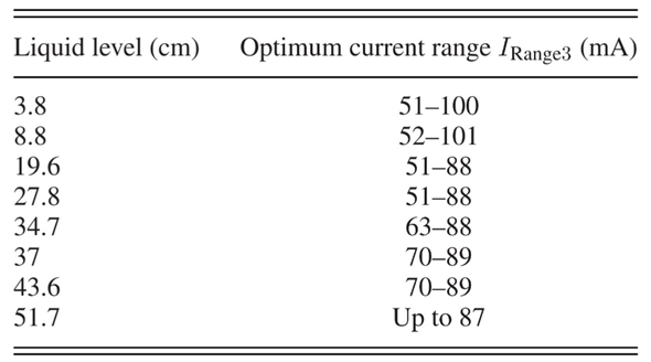
The optimum current also varies with the liquid level inside the vessel or cryostat as shown in table 4 which represents the optimum current range found for different liquid levels with a NbTi wire. It should lie within the overlap of the found optimum current ranges for all liquid levels. In the shown example, 75 mA was selected as the optimum current.
Table 4: Example: Optimum current ranges for different liquid levels from [2].
As explained above, the helium probe must be used with an appropriate current (“optimum current”) to get measuring results which correspond correctly to the liquid helium level. To obtain this optimum current, two steps must be followed for different filling levels of the vessel:
- Scan the liquid helium probe resistance with the “linear” pulse of the pulse menu for a wide range of current values to find the (optimum) current range with constant resistance.
- Verify the found optimum current range with the “constant” pulse of the pulse menu.
These two steps are illustrated by figures in the following.
1. Scan liquid helium probe with “linear” pulse type
The HZB level meter has a built-in function (“linear” pulse type in the pulse menu of the diagnosis mode) which offers the possibility to scan the probe for its resistance over a wide range of current values. An example is shown in fig. 18.
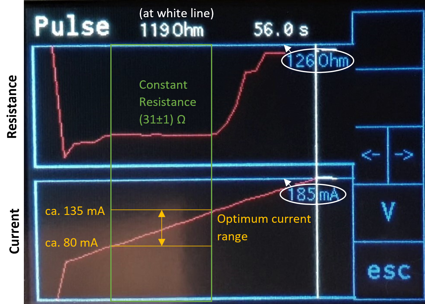
Figure 18: Analyzing a liquid helium probe with the „linear“ pulse type of the pulse menu which can be opened via the diagnosis menu of the helium level meter. The lower diagram shows the current values over the time which are set during the measurements. The upper diagram shows the corresponding measured values of the probe resistance. The parameters of this measurement were: I min=60 mA, I max=185 mA, Delta I=5 mA and Delta t=2 s. The found optimum current range is marked.
As explained above, the not-superconducting part of the helium probe gets to a certain height depending on the current. If the current is too low, a certain length of the probe above the vapor liquid interface remains in the superconducting state. If the current is too high, the not-superconducting part of the probe reaches below the interface. In between, there is a range of current which lets the not-superconducting part begin exactly at the interface. This height occurs as a range of constant resistance which is marked green in fig. 18. The corresponding current range (marked yellow) is the wanted optimum current range.
The first scan usually should scan over a wide range of current with a relatively rough resolution. Hence, these measurements should be reiterated, this time for current ranges around the left and the right boundary of the found optimum current range. In this case, measurements from 70 mA to 86 mA (left boundary) and from 125 mA to 145 mA (right boundary) are performed with steps of 1 mA. These resistance measurements are shown in fig. 19 and 20. We have found that the measurements are reliable even for low Delta t of about 1 s, thus it can be set to this value.
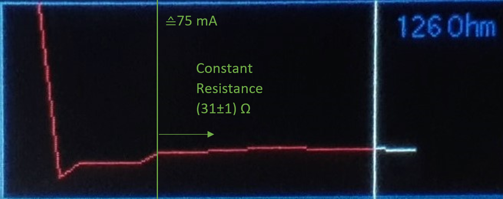
Figure 19: Scan at the found left boundary of the optimum current range with I min=70 mA, I max=86 mA, Delta I=1 mA and Delta t=1 s. Only the resistance diagram is shown. The max. value at the upper boundary of the diagram is 126 Ohm. The green line marks the left boundary of the constant resistance range. This corresponds to a current of 75 mA.
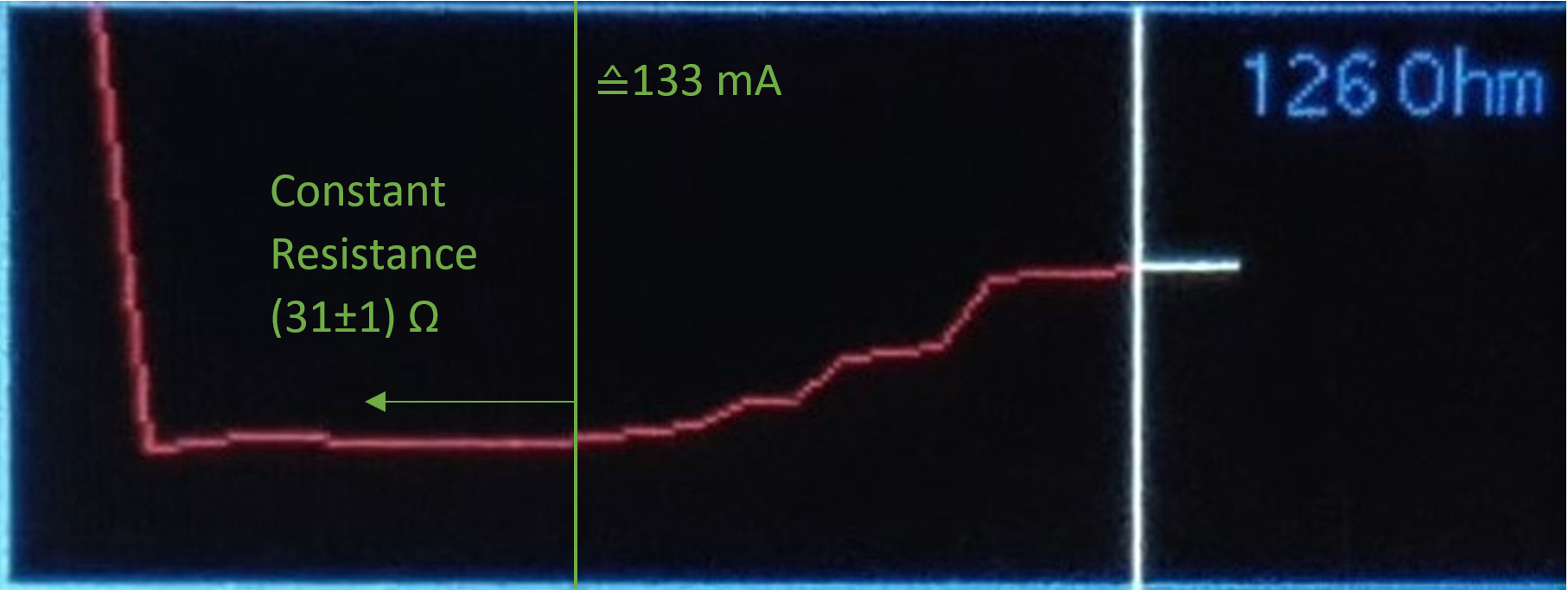
Figure 20: Scan at the found right boundary of the optimum current range with I min=125 mA, I max=145 mA, Delta I=1 mA and Delta t=4 s. Only the resistance diagram is shown. The max. value at the upper boundary of the diagram is 126 Ohm. The green line marks the right boundary of the constant resistance range. This corresponds to a current of 133 mA.
Using the “linear” pulse type, the boundaries of the optimum current range are found. These values should be verified by using the “constant” pulse type in the following.
2. Verify the found optimum current range with the “constant” pulse type
To verify the found boundaries, measurements using the “constant” pulse type of the pulse menu should be performed. This measurement applies a constant current to the probe and measures the resistance over time. Measurements at the left boundary are shown in fig. 21.
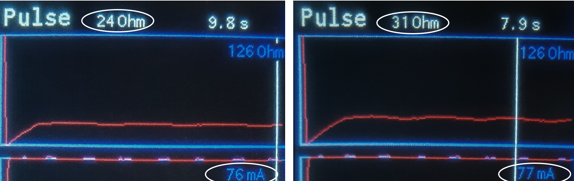
Figure 21: Measurements at the left boundary of the found optimum current range using the „constant“ pulse type with a duration of 10 s. The left measurement uses a constant current of 76 mA and reaches after some seconds a resistance of 24 Ohm. The right diagram shows the same measurement with a constant current of 77 mA. In this case, the resistance reaches 31 Ohm which is the value of the optimum current range, found before. This shows that the optimum current range begins exactly at 77 mA.
A measurement using the “constant” pulse type in the center of the optimum current range verifies the previously found constant resistance in this range. This is shown in fig. 22.
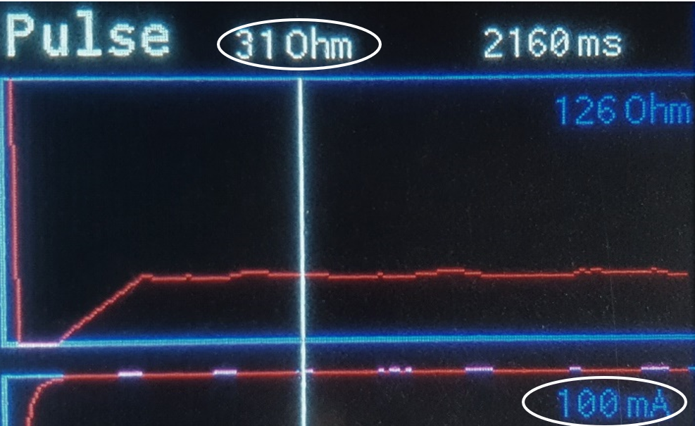
Figure 22: Verifying the resistance in the optimum current range found previously. Using the „constant“ pulse type with 100 mA, the resistance of 31 Ohm can be confirmed.
After having found that the left boundary lies at 77 mA which is close to the 75 mA, previously found with the “linear” pulse type, and having confirmed the resistance in the optimum current range at 31 Ohm, also the right boundary should be examined using the “constant” pulse type. This is shown in fig. 23.
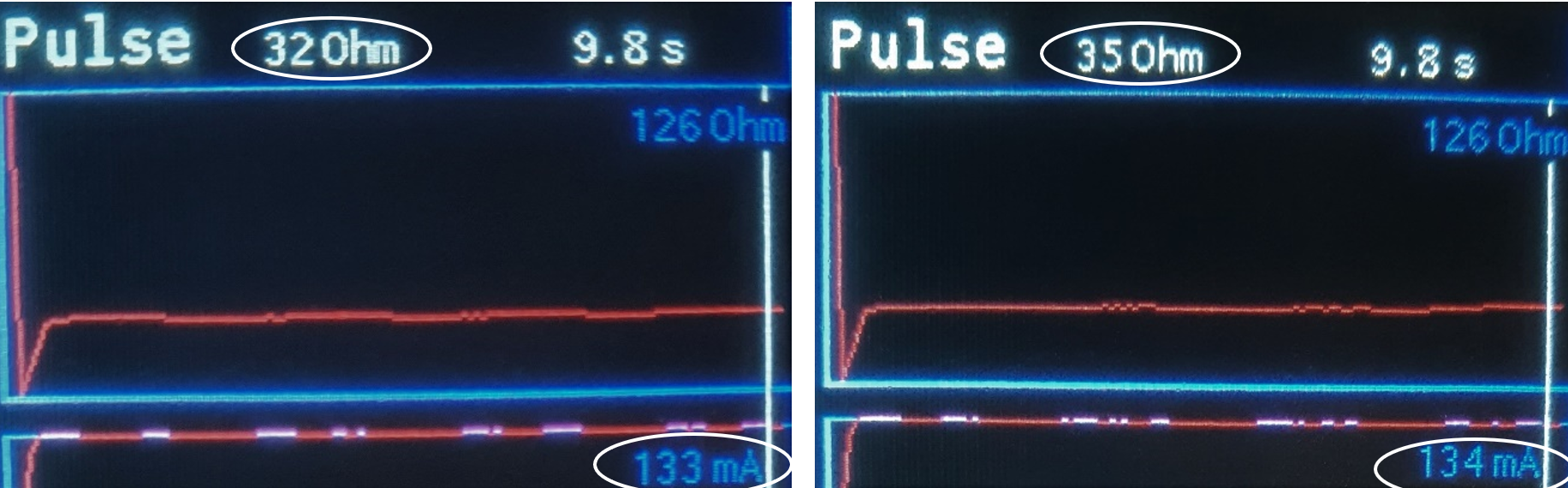
Figure 23: Examining the right boundary of the found optimum current range using the „constant“ pulse type. The resistance slightly increases at 134 mA which confirms the previously found right boundary of 133 mA.
The resistance increases at 134 mA to 35 Ohm which lies above the resistance found in the optimum current range. This confirms the previously found right boundary of the optimum current range at 133 mA. Also look onto the time needed for reaching the plateau. This will be used as waiting time in the measurement settings.
Result of the Examinations and Further Proceedings
The optimum current range is found to be between 77 mA and 133 mA for the given liquid level of the examined liquid helium vessel. This can be different for another liquid level (see table 4). Thus, the procedure described here should be performed for a high liquid helium level and a low one and the overlap of the found two optimum current ranges defines the new optimum current range. For example, when you find the optimum current range at low liquid helium level to be from 90 mA to 150 mA, the resulting optimum current range for all liquid levels would be from 90 mA to 133 mA.
A current value within the new optimum current range can be used for reliable measurements of the liquid helium level. To reduce the heat input into the vessel or cryostat, a smaller current within this range should be selected as the optimum current value. For shorter measurement time and for working at higher boil-off rates a higher current value should be selected. A compromise for the optimum current value lies at about the lower one third of the found optimum current range. In the given example, the optimum current value would lie at the lower one third between 90 and 133 mA which is 104 mA.
The time spans found in the “constant” mode measurements which reflect the time needed to heat the upper part of the probe to the normal conducting state, must be considered. The largest value of this time span – typically achieved for a relatively empty vessel – should be used in the following as waiting time before beginning the level measurements.
Cooking Recipe for Determining the Optimum Current Value
- Repeat for at least a high and a low liquid helium level in the vessel:
- Use the “linear” pulse type in the pulse menu accessible via the diagnosis mode for scanning the probes resistance over a wide range of currents (e.g. 0 mA to 200 mA). A Delta t of 1 s typically should be enough for the scan. Identify the plateau in the resistance curve which corresponds to the optimum current range. Use the cursor line to display the resistance value in this range. Attention: the highest value reached typically corresponds to the probe being completely not superconducting. This also produces a plateau at high resistance values.
- Use again the “linear” pulse type to verify the found boundaries of the optimum current range (plateau). Scan with 1 mA steps around the left and the right boundary.
- Verify the found boundaries by using the “constant” pulse type which applies for a given duration a constant current to the probe. At first, check the found resistance value in the optimum current range. Then, use current values at the found boundaries of the optimum current range and examine which resistance values are reached after some seconds. The correct boundaries are the lowest and the highest current values which result in the resistance value found in the optimum current range. Also observe the time needed to reach the resistance plateau.
- Build the overlap of the found optimum current ranges for different liquid helium levels (e.g. at high level 77 mA – 133 mA and at low level 90 mA – 150 mA results in an overlap of 90 mA – 133 mA). Considering advantages and disadvantages, the optimum current value of interest is at about the lower one third within this range. In the given example, the optimum current is 104 mA. The largest time span needed to heat up the probe in step 1c is used as waiting time later.
The values to enter on options page 2 which will be used for measurements of the liquid helium level characterize a measurement using the two-current approach, mentioned above. This can be modified to perform measurements using the one-current approach by changing “Pulse” to 0.0 seconds. Then, the “Wait” time describes the time of heating up the upper part of the probe until starting the measurement of the level. The largest time span needed for reaching the resistance plateau using the “constant” pulses (in cooking recipe step 1c) should be set as the waiting time. “I meas” is the current which is used for the measurements and should be set to the previously found optimum current value.
Nevertheless, the two-current approach can be useful in case of a lacking small resistor (external heater) at the top of the liquid helium probe. This can result in the problem that a completely superconducting probe typically at high liquid helium levels wrongly yields unchangeable 0 Ohm (or a few Ohm due to resistance of feeding lines) because no warm starting point can be generated. In this case, a high current can help to quench the probe and to obtain reasonable values. Another advantage of a higher current at beginning of the measurement is that less time is needed for taking the measurement due to the faster heating of the probe. You can validate the settings of the two-current measurements by comparing the result with that obtained by the previously mentioned “constant” pulse type using the optimum current value
In order to obtain the resistance values corresponding to filling levels of 100% and 0% (minimum and maximum resistance, respectively), measurements of the probe must be performed in a relatively full vessel or cryostat. For this purpose, the “constant” pulse type, accessible via the pulse menu inside the diagnosis mode should be used. The minimum resistance can be found by applying a very low current to the probe according to the current range 1 in fig. 16. It is possible that this value is not zero due to the remaining resistance of the feeding lines, for example. The minimum resistance corresponds to a full vessel or cryostat with 100% liquid level. The maximum resistance can be found by applying a high current to the probe according to the current range 5 in fig. 16. This means that the whole probe is brought into the normal conducting state. The maximum resistance corresponds to an empty vessel or cryostat with 0% liquid level.
These values must be entered on page 3 of the options menu to complete the setup process of the liquid helium probe. Moreover, the filling level is foreseen to be weighted by the shape of the vessel or cryostat to obtain the liquid volume in the vessel.
Attention: The maximum resistance obtained this way can differ significantly from the real resistance of the empty vessel (we obtained up to 20% above the ideal value), presumably caused by strong warming of the superconducting wire. Check the value by observing the liquid helium level of the nearly empty vessel over time. When the level in percent stagnates, this should be near 0%. Otherwise, the maximum resistance is wrong and should be corrected. A plateau above 0% implies that the maximum resistance must be corrected upwards, a plateau below 0% means that it should be corrected downwards.
[1] M. Takeda, Y. Inoue, K. Maekawa, Y. Matsuno, S. Fujikawa, and H. Kumakura, “Superconducting characteristics of short MgB2 wires of long level sensor for liquid hydrogen,” in Proc. IOP Conf. Series, Mater. Sci. Eng., 2015, vol. 101, Paper 012156.
[2] K.R. Kunniyoor, T. Richter, P. Ghosh, R. Lietzow, S. Schlachter, and H. Neumann, “Experimental Study on Superconducting Level Sensors in Liquid Helium”, IEEE Trans. Appl. Supercond., vol. 28, no. 2, March 2018, Art. no. 9000810.
[3] K. R. Kunniyoor, T. Richter, P. Ghosh, R. Lietzow, and H. Neumann, “A Mathematical Model for the Characterization of Superconducting Level Sensors”, IEEE Trans. Appl. Supercond., vol. 28, no. 1, Jan. 2018, Art. no. 9000111.